The goal of BayesianPlatformDesignTimeTrend is to simulates the multi-arm multi-stage or platform trial with Bayesian approach using the ‘rstan’ package, which provides the R interface for to the stan. The package uses Thall’s and Trippa’s randomisation approach for Bayesian adaptive randomisation. In addition, the time trend problem of platform trial can be studied in this package. There are a some demos for the simulation process of cutoff screening, hyperprameter tuning and design evaluation in this package.
You can install the ‘BayesianPlatformDesignTimeTrend’ package 1.2.0 like so:
# install.packages("BayesianPlatformDesignTimeTrend")
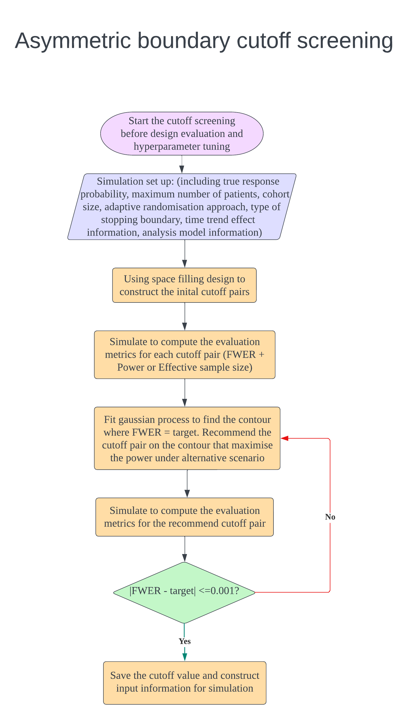
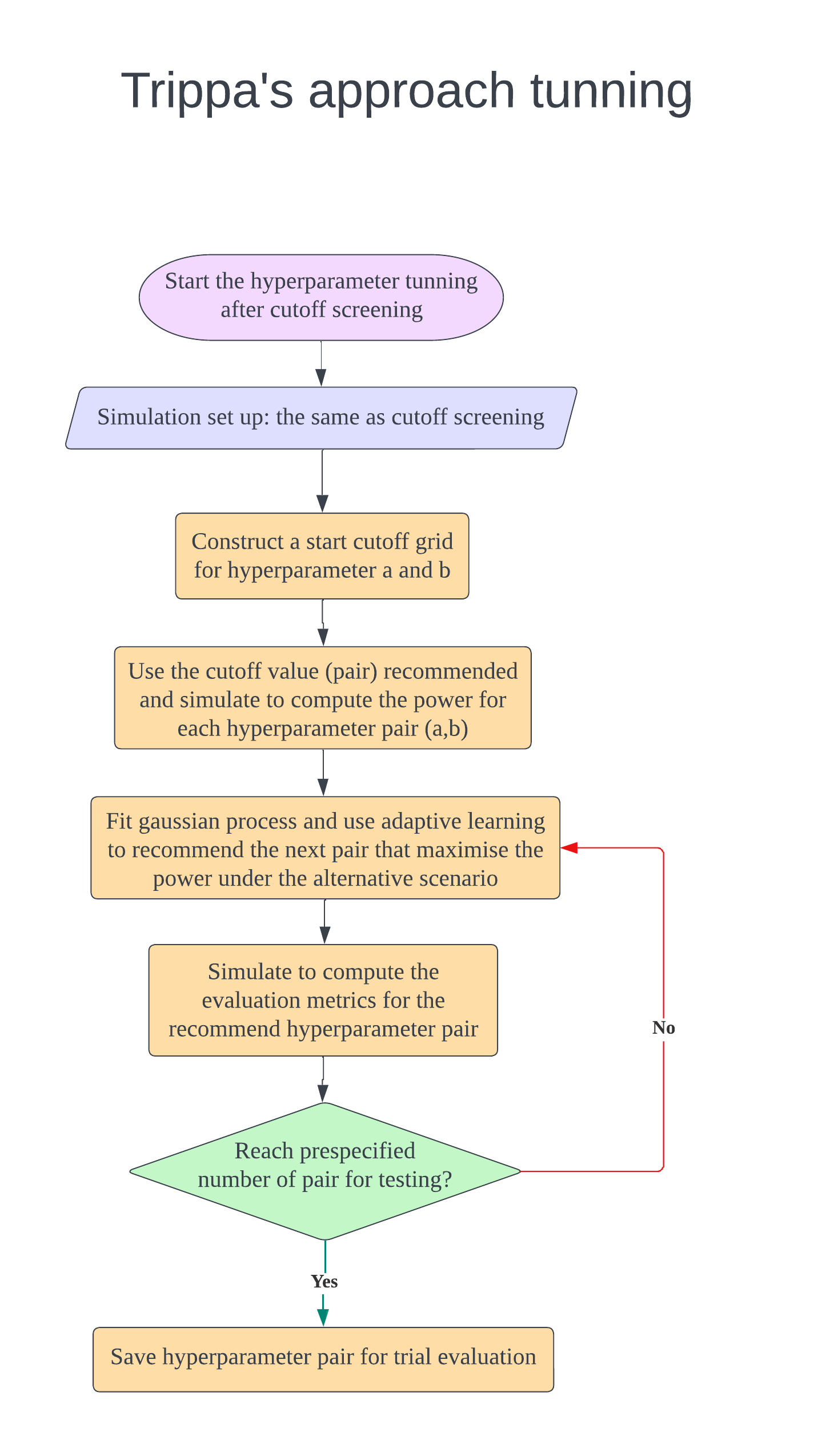
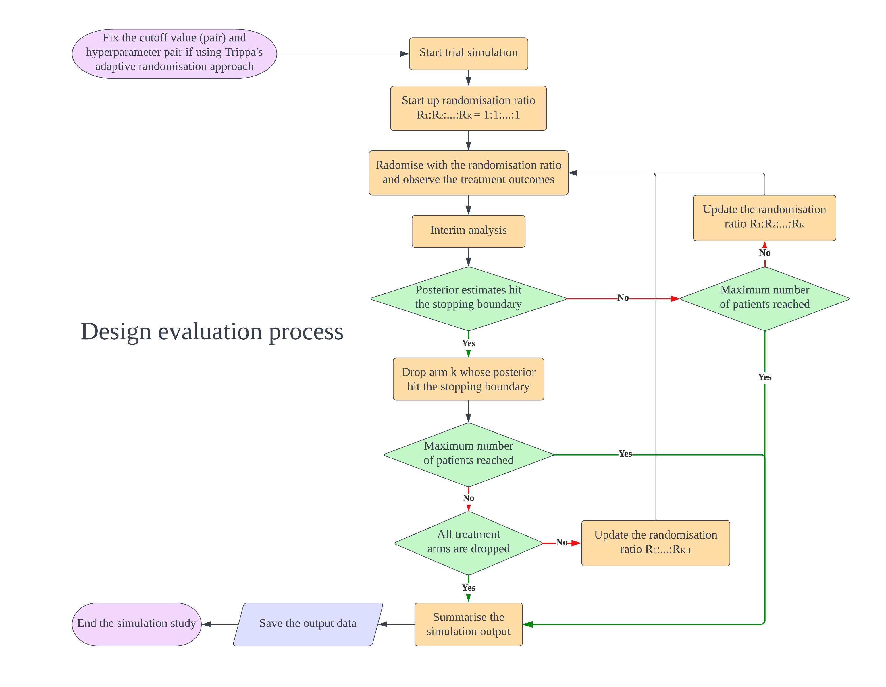
# devtools::install_github("ZXW834/BayesianPlatformDesignTimeTrend", build_vignettes = TRUE)In the design, \(K\) intervention arms are evaluated compared to a shared control. During the trial, there are several interim analyses for decision making to claim superiority of each arm (Oneside test) or both inferiority and superiority of each arm (Twoside test). There are several parameters can be tuned which are cutoff values of stopping boundaries and the hyperparameters of Trippa’s adaptive randomisation approach. The below figures illustrate how to do design evaluation using this package. We need to set up the design first and start with cutoff screening to control the FWER and maximise the power. If the investigator want to tune hyperparameters of Trippa’s approach to maximise the power further, the randomisation method in cutoff screening process should be adaptive randomisation (Eg.Thall’s approach). We found that after fixing the cutoff value, the change of adaptive randomisation method does not inflate the FWER. After finding the cutoff (and hyperparameter), the design is fixed and can be evaluated. If investigator wants to compare the design with different maximum sample size, just use the same cutoff (and hyperparameter) and only change the sample size parameter to create a new design for evaluation.
Demo_CutoffScreening() is a demo function performing cutoff screening process where simple linear model is fitDemo_CutoffScreening_GP() is a demo function performing cutoff screening process where Gaussian process is fit and active learning is usedDemo_multiplescrenariotrialsimulation() is a demo function performing MAMS trial simulationMAMS-CutoffScreening-tutorial is a tutorial document of how to do cutoff screening under Bayesian MAMS trial fitting linear model.MAMS-CutoffScreening-GP-Asymmetric-tutorial is a tutorial document of how to do symmetric cutoff screening under Bayesian MAMS trial fitting the Gaussian process.MAMS-CutoffScreening-GP-Symmetric-tutorial is a tutorial document of how to do asymmetric cutoff screening under Bayesian MAMS trial fitting the Gaussian process.MAMS-trial-simulation-tutorial is a tutorial document of how to do Bayesian MAMS trial simulation with or without time trend.This is a basic example which shows you how to solve a common problem:
output=Trial.simulation(ntrials = 10000,
trial.fun = simulatetrial,
 input.info = list(
   response.probs = c(0.4, 0.4),
   ns = c(60, 120, 180, 240, 300),
   max.ar = 0.75,
   rand.algo = "Urn",
   max.deviation = 3,
   model.inf = list(
     model = "tlr",
     ibb.inf = list(
       pi.star = 0.5,
       pess = 2,
       betabinomialmodel = ibetabinomial.post
     ),
     tlr.inf = list(
       beta0_prior_mu = 0,
       beta1_prior_mu = 0,
       beta0_prior_sigma = 2.5,
       beta1_prior_sigma = 2.5,
       beta0_df = 7,
       beta1_df = 7,
       reg.inf =  "main",
       variable.inf = "Fixeffect"
     )
   ),
   Stopbound.inf = Stopboundinf(
     Stop.type = "Early-Pocock",
       Boundary.type = "Symmetric",
         cutoff = c(0.9925, 0.0075)
         ),
   Random.inf = list(
     Fixratio = FALSE,
     Fixratiocontrol = NA,
     BARmethod = "Thall",
     Thall.tuning.inf = list(tuningparameter = "Fixed",  fixvalue = 1)
   ),
   trend.inf = list(
     trend.type = "step",
     trend.effect = c(0, 0),
     trend_add_or_multip = "mult"
   )
 ),
 cl = 2)
Here is the operational characteristics table for previous single null scenario simulation.