![]()
![]()
![]()
![]()


![]()
This package estimates the time-varying reproduction number, growth rate, and doubling time using a range of open-source tools (Abbott et al.), and current best practices (Gostic et al.). It aims to help users avoid some of the limitations of naive implementations in a framework that is informed by community feedback and is actively supported.
It estimates the time-varying reproduction number on cases by date of
infection (using a similar approach to that implemented in {EpiEstim}).
Imputed infections are then mapped to observed data (for example cases
by date of report) via a series of uncertain delay distributions (in the
examples in the package documentation these are an incubation period and
a reporting delay) and a reporting model that can include weekly
periodicity.
Uncertainty is propagated from all inputs into the final parameter estimates, helping to mitigate spurious findings. This is handled internally. The time-varying reproduction estimates and the uncertain generation time also give time-varying estimates of the rate of growth.
The default model uses a non-stationary Gaussian process to estimate the time-varying reproduction number and then infer infections. Other options include:
These options generally reduce runtimes at the cost of the granularity of estimates or at the cost of real-time performance.
The documentation for estimate_infections
provides examples of the implementation of the different options
available.
Forecasting is also supported for the time-varying reproduction number, infections and reported cases using the same generative process approach as used for estimation.
A simple example of using the package to estimate a national Rt for Covid-19 can be found here.
EpiNow2 also supports adjustment for truncated data via
estimate_truncation() (though users may be interested in
more flexibility and if so should check out the epinowcast
package), and for estimating dependent observations (i.e deaths based on
hospital admissions) using estimate_secondary().
Install the released version of the package:
install.packages("EpiNow2")Install the development version of the package with:
install.packages("EpiNow2", repos = "https://epiforecasts.r-universe.dev")Alternatively, install the development version of the package with pak as follows (few users should need to do this):
# check whether {pak} is installed
if (!require("pak")) {
  install.packages("pak")
}
pak::pkg_install("epiforecasts/EpiNow2")
If using pak fails, try:
# check whether {remotes} is installed
if (!require("remotes")) {
  install.packages("remotes")
}
remotes::install_github("epiforecasts/EpiNow2")
Windows users will need a working installation of Rtools in order to build the package from source. See here for a guide to installing Rtools for use with Stan (which is the statistical modelling platform used for the underlying model). For simple deployment/development a prebuilt docker image is also available (see documentation here).
{EpiNow2} is designed to be used with a single function
call or to be used in an ad-hoc fashion via individual function calls.
The core functions of {EpiNow2} are the two single-call
functions epinow(),
regional_epinow(),
plus functions estimate_infections(),
estimate_secondary()
and estimate_truncation().
In the following section we give an overview of the simple use case for
epinow and regional_epinow. estimate_infections()
can be used on its own to infer the underlying infection case curve from
reported cases and estimate Rt. Estimating the underlying infection case
curve via back-calculation (and then calculating Rt) is substantially
less computationally demanding than generating using default settings
but may result in less reliable estimates of Rt. For more details on
using each function see the function
documentation.
The first step to using the package is to load it as follows.
library(EpiNow2)Distributions can either be fitted using package functionality or
determined elsewhere and then defined with uncertainty for use in
{EpiNow2}. When data is supplied a subsampled bootstrapped
lognormal will be fit (to account for uncertainty in the observed data
without being biased by changes in incidence). An arbitrary number of
delay distributions are supported with the most common use case likely
to be a incubation period followed by a reporting delay.
For example if data on the delay between onset and infection was available we could fit a distribution to it with appropriate uncertainty as follows (note this is a synthetic example),
reporting_delay <- estimate_delay(
  rlnorm(1000, log(2), 1),
  max_value = 15, bootstraps = 1
)
If data was not available we could instead make an informed estimate of the likely delay (this is a synthetic example and not applicable to real world use cases and we have not included uncertainty to decrease runtimes),
reporting_delay <- dist_spec(
  mean = convert_to_logmean(2, 1), sd = convert_to_logsd(2, 1), max = 10,
  dist = "lognormal"
)
Here we define the incubation period and generation time based on literature estimates for Covid-19 (see here for the code that generates these estimates). Note that these distributions may not be applicable for your use case and that we have not included uncertainty here to reduce the runtime of this example but in most settings this is not recommended.
generation_time <- get_generation_time(
  disease = "SARS-CoV-2", source = "ganyani", max = 10, fixed = TRUE
)
incubation_period <- get_incubation_period(
  disease = "SARS-CoV-2", source = "lauer", max = 10, fixed = TRUE
)This function represents the core functionality of the package and includes results reporting, plotting and optional saving. It requires a data frame of cases by date of report and the distributions defined above.
Load example case data from {EpiNow2}.
reported_cases <- example_confirmed[1:60]
head(reported_cases)
#>          date confirm
#> 1: 2020-02-22      14
#> 2: 2020-02-23      62
#> 3: 2020-02-24      53
#> 4: 2020-02-25      97
#> 5: 2020-02-26      93
#> 6: 2020-02-27      78
Estimate cases by date of infection, the time-varying reproduction
number, the rate of growth and forecast these estimates into the future
by 7 days. Summarise the posterior and return a summary table and plots
for reporting purposes. If a target_folder is supplied
results can be internally saved (with the option to also turn off
explicit returning of results). Here we use the default model
parameterisation that prioritises real-time performance over run-time or
other considerations. For other formulations see the documentation for
estimate_infections().
estimates <- epinow(
  reported_cases = reported_cases,
  generation_time = generation_time_opts(generation_time),
  delays = delay_opts(incubation_period + reporting_delay),
  rt = rt_opts(prior = list(mean = 2, sd = 0.2)),
  stan = stan_opts(cores = 4, control = list(adapt_delta = 0.99)),
  verbose = interactive()
)
names(estimates)
#> [1] "estimates"                "estimated_reported_cases"
#> [3] "summary"                  "plots"
#> [5] "timing"
Both summary measures and posterior samples are returned for all
parameters in an easily explored format which can be accessed using
summary. The default is to return a summary table of
estimates for key parameters at the latest date partially supported by
data.
knitr::kable(summary(estimates))| measure | estimate |
|---|---|
| New confirmed cases by infection date | 2313 (1159 – 4345) |
| Expected change in daily cases | Likely decreasing |
| Effective reproduction no. | 0.89 (0.62 – 1.2) |
| Rate of growth | -0.026 (-0.1 – 0.038) |
| Doubling/halving time (days) | -26 (18 – -6.7) |
Summarised parameter estimates can also easily be returned, either filtered for a single parameter or for all parameters.
head(summary(estimates, type = "parameters", params = "R"))
#>          date variable strat     type   median     mean         sd lower_90
#> 1: 2020-02-22        R    NA estimate 2.140044 2.142893 0.13818099 1.937615
#> 2: 2020-02-23        R    NA estimate 2.105628 2.106892 0.11415164 1.936612
#> 3: 2020-02-24        R    NA estimate 2.068985 2.069442 0.09420757 1.921287
#> 4: 2020-02-25        R    NA estimate 2.031434 2.030725 0.07830576 1.907767
#> 5: 2020-02-26        R    NA estimate 1.991226 1.990969 0.06634858 1.884688
#> 6: 2020-02-27        R    NA estimate 1.950962 1.950427 0.05807390 1.856440
#>    lower_50 lower_20 upper_20 upper_50 upper_90
#> 1: 2.046299 2.104219 2.174057 2.232616 2.370781
#> 2: 2.025782 2.075403 2.132810 2.182697 2.294095
#> 3: 2.003747 2.044222 2.090967 2.131610 2.225019
#> 4: 1.977390 2.010528 2.048636 2.082264 2.163819
#> 5: 1.944677 1.974170 2.008207 2.035011 2.103163
#> 6: 1.910567 1.935790 1.965265 1.988672 2.046538
Reported cases are returned in a separate data frame in order to streamline the reporting of forecasts and for model evaluation.
head(summary(estimates, output = "estimated_reported_cases"))
#>          date  type median     mean       sd lower_90 lower_50 lower_20
#> 1: 2020-02-22 gp_rt   65.5  67.2870 18.83096       40       54       61
#> 2: 2020-02-23 gp_rt   78.0  78.8395 21.73755       47       63       72
#> 3: 2020-02-24 gp_rt   77.0  78.8920 21.59142       47       64       72
#> 4: 2020-02-25 gp_rt   73.0  75.0705 20.82804       45       61       68
#> 5: 2020-02-26 gp_rt   78.0  79.8325 22.03166       47       65       73
#> 6: 2020-02-27 gp_rt  110.0 112.9160 28.92359       71       92      103
#>    upper_20 upper_50 upper_90
#> 1:       70    79.00      101
#> 2:       83    92.00      117
#> 3:       82    92.00      116
#> 4:       78    87.00      115
#> 5:       83    91.25      120
#> 6:      118   130.00      165
A range of plots are returned (with the single summary plot shown
below). These plots can also be generated using the following
plot method.
plot(estimates)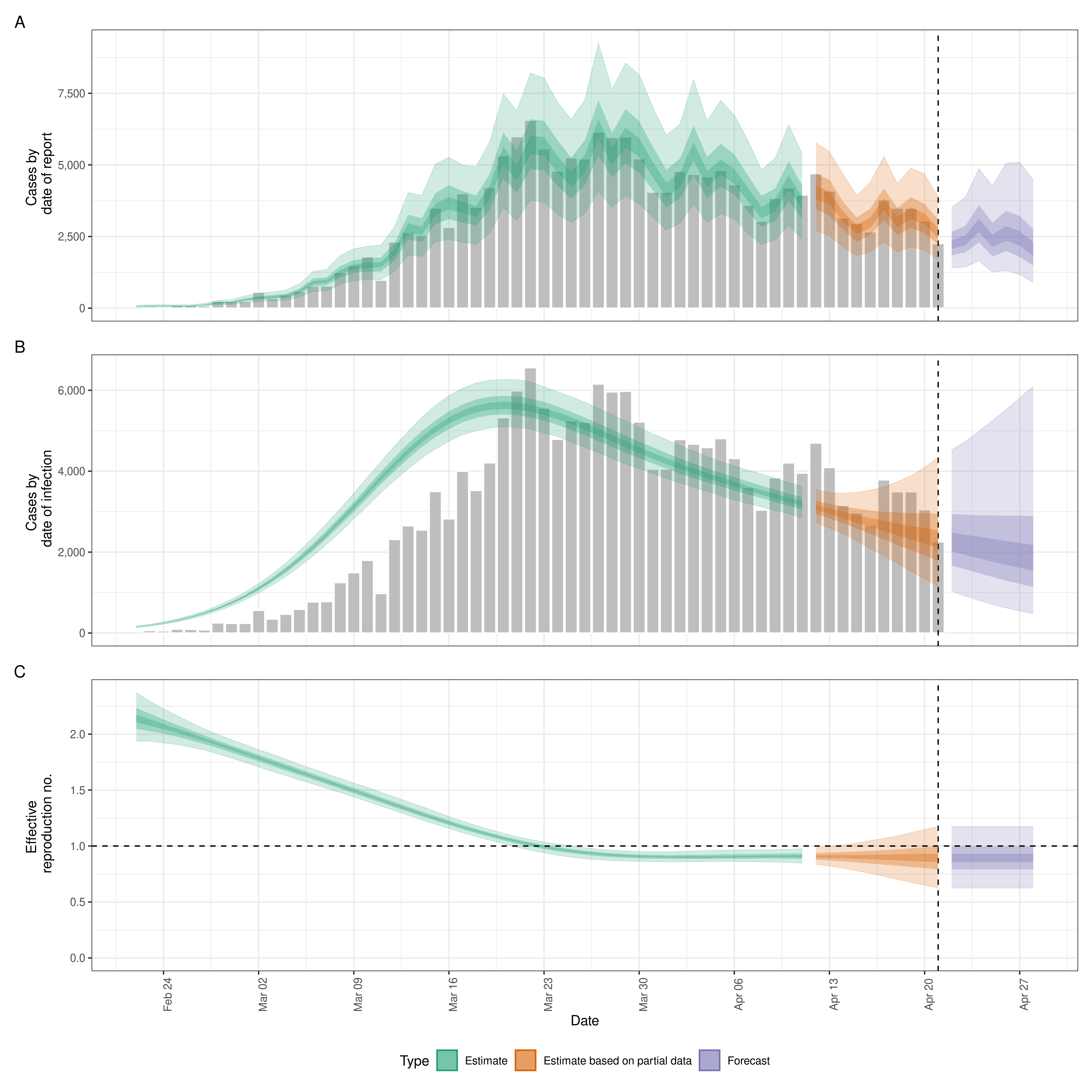
The regional_epinow() function runs the
epinow() function across multiple regions in an efficient
manner.
Define cases in multiple regions delineated by the region variable.
reported_cases <- data.table::rbindlist(list(
  data.table::copy(reported_cases)[, region := "testland"],
  reported_cases[, region := "realland"]
))
head(reported_cases)
#>          date confirm   region
#> 1: 2020-02-22      14 testland
#> 2: 2020-02-23      62 testland
#> 3: 2020-02-24      53 testland
#> 4: 2020-02-25      97 testland
#> 5: 2020-02-26      93 testland
#> 6: 2020-02-27      78 testland
Calling regional_epinow() runs the epinow()
on each region in turn (or in parallel depending on the settings used).
Here we switch to using a weekly random walk rather than the full
Gaussian process model giving us piecewise constant estimates by
week.
estimates <- regional_epinow(
  reported_cases = reported_cases,
  generation_time = generation_time_opts(generation_time),
  delays = delay_opts(incubation_period + reporting_delay),
  rt = rt_opts(prior = list(mean = 2, sd = 0.2), rw = 7),
  gp = NULL,
  stan = stan_opts(cores = 4, warmup = 250, samples = 1000)
)
#> INFO [2023-06-09 13:52:11] Producing following optional outputs: regions, summary, samples, plots, latest
#> INFO [2023-06-09 13:52:11] Reporting estimates using data up to: 2020-04-21
#> INFO [2023-06-09 13:52:11] No target directory specified so returning output
#> INFO [2023-06-09 13:52:11] Producing estimates for: testland, realland
#> INFO [2023-06-09 13:52:11] Regions excluded: none
#> INFO [2023-06-09 13:52:40] Completed estimates for: testland
#> INFO [2023-06-09 13:53:07] Completed estimates for: realland
#> INFO [2023-06-09 13:53:07] Completed regional estimates
#> INFO [2023-06-09 13:53:07] Regions with estimates: 2
#> INFO [2023-06-09 13:53:07] Regions with runtime errors: 0
#> INFO [2023-06-09 13:53:07] Producing summary
#> INFO [2023-06-09 13:53:07] No summary directory specified so returning summary output
#> INFO [2023-06-09 13:53:08] No target directory specified so returning timings
Results from each region are stored in a regional list
with across region summary measures and plots stored in a
summary list. All results can be set to be internally saved
by setting the target_folder and summary_dir
arguments. Each region can be estimated in parallel using the
{future} package (when in most scenarios cores
should be set to 1). For routine use each MCMC chain can also be run in
parallel (with future = TRUE) with a time out
(max_execution_time) allowing for partial results to be
returned if a subset of chains is running longer than expected. See the
documentation for the {future} package for details on
nested futures.
Summary measures that are returned include a table formatted for reporting (along with raw results for further processing). Futures updated will extend the S3 methods used above to smooth access to this output.
knitr::kable(estimates$summary$summarised_results$table)| Region | New confirmed cases by infection date | Expected change in daily cases | Effective reproduction no. | Rate of growth | Doubling/halving time (days) |
|---|---|---|---|---|---|
| realland | 2176 (1192 – 4065) | Likely decreasing | 0.87 (0.65 – 1.1) | -0.032 (-0.096 – 0.03) | -22 (23 – -7.2) |
| testland | 2217 (1150 – 4155) | Likely decreasing | 0.87 (0.64 – 1.2) | -0.031 (-0.099 – 0.036) | -23 (19 – -7) |
A range of plots are again returned (with the single summary plot shown below).
estimates$summary$summary_plot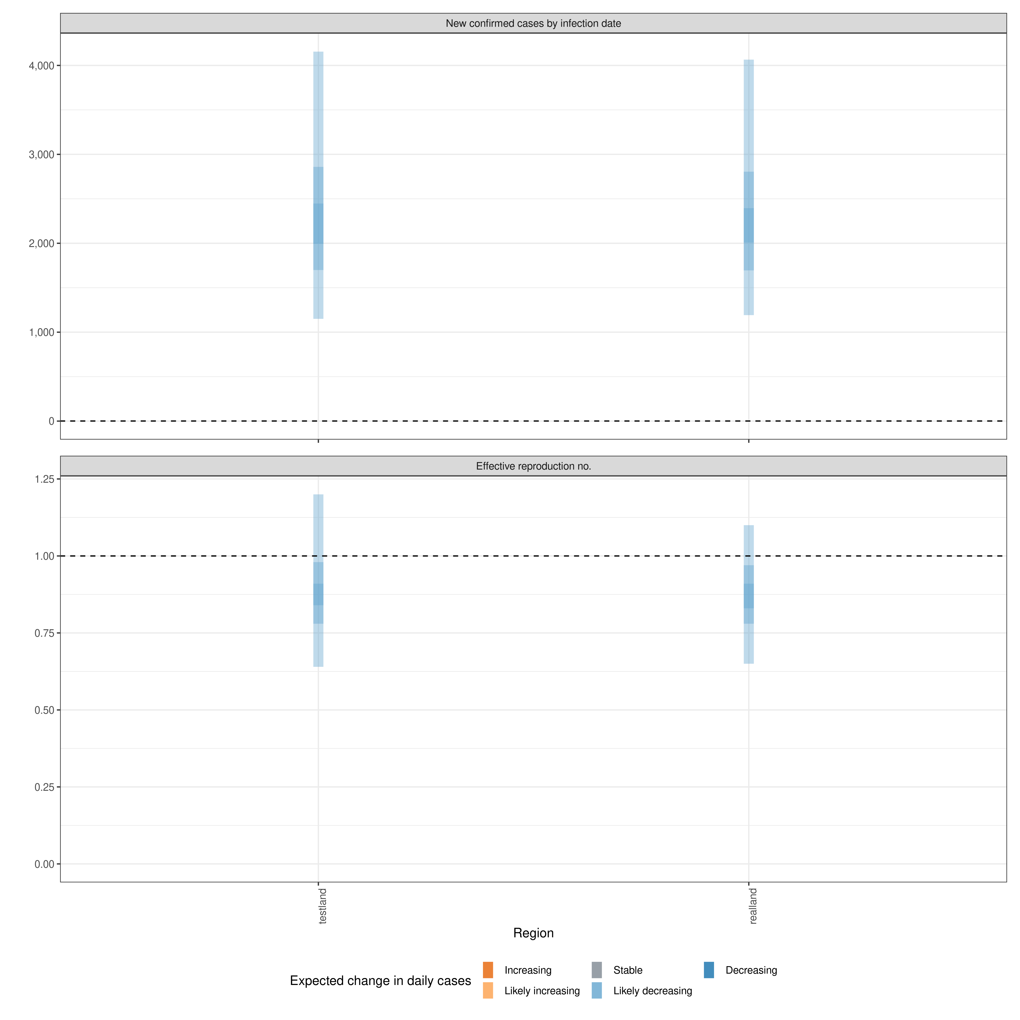
Rmarkdown templates are provided in the package
(templates) for semi-automated reporting of estimates. If
using these templates to report your results please highlight our limitations
as these are key to understanding the results from
{EpiNow2} .
File an issue here if you have identified an issue with the package. Please note that due to operational constraints priority will be given to users informing government policy or offering methodological insights. We welcome all contributions, in particular those that improve the approach or the robustness of the code base. We also welcome additions and extensions to the underlying model either in the form of options or improvements.