arctools package to compute physical activity summaries
activity_stats
method options
activity_stats method
![]()
The arctools package allows to generate summaries of the
minute-level physical activity (PA) data. The default parameters are
chosen for the Actigraph activity counts collected with a wrist-worn
device; however, the package can be used for other minute-level PA data
with the corresponding timepstamps vector.
Below, we demonstrate the use of arctools with the
attached, exemplary minute-level Actigraph PA counts data.
You can install the released version of arctools from GitHub. Note you may need to install
devtools package if not yet installed (the line commented
below).
# install.packages("devtools")
devtools::install_github("martakarass/arctools")A PDF with detailed documentation of all methods can be accessed here.
arctools package to compute physical activity
summariesFour CSV data sets with minute-level activity counts data are
attached to the arctools package. The data file names are
stored in extdata_fnames object that becomes available once
the arctools package is loaded.
library(arctools)
library(data.table)
library(dplyr)
library(lubridate)
library(ggplot2)

## Read one of the data sets
fpath <- system.file("extdata", extdata_fnames[1], package = "arctools")
dat   <- as.data.frame(fread(fpath))
rbind(head(dat, 3), tail(dat, 3))
#>       Axis1 Axis2 Axis3 vectormagnitude           timestamp
#> 1      1021  1353  2170            2754 2018-07-13 10:00:00
#> 2      1656  1190  2212            3009 2018-07-13 10:01:00
#> 3      2540  1461  1957            3524 2018-07-13 10:02:00
#> 10078     0     0     0               0 2018-07-20 09:57:00
#> 10079     0     0     0               0 2018-07-20 09:58:00
#> 10080     0     0     0               0 2018-07-20 09:59:00
The data columns are:
Axis1 - sensor’s X axis minute-level counts data,Axis2 - sensor’s Y axis minute-level counts data,Axis3 - sensor’s Z axis minute-level counts data,vectormagnitude - minute-level counts data defined as
sqrt(Axis1^2 + Axis2^2 + Axis3^2),timestamp - time-stamps corresponding to minute-level
measures.## Plot activity counts
## Format timestamp data column from character to POSIXct object
ggplot(dat, aes(x = ymd_hms(timestamp), y = vectormagnitude)) +
geom_line(size = 0.3, alpha = 0.8) +
labs(x = "Time", y = "Activity counts") +
theme_gray(base_size = 10) +
scale_x_datetime(date_breaks = "1 day", date_labels = "%b %d")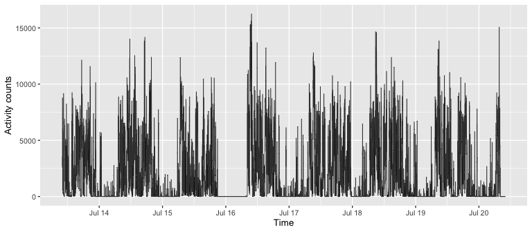
activity_stats methodacc <- dat$vectormagnitude
acc_ts <- ymd_hms(dat$timestamp)
activity_stats(acc, acc_ts)
#> n_days n_valid_days wear_time_on_valid_days tac tlac ltac
#> 1 8 4 1440 2826648 6429.838 14.8546
#> astp satp time_spent_active time_spent_nonactive
#> 1 0.1781782 0.09516215 499.5 940.5
#> no_of_active_bouts no_of_nonactive_bouts mean_active_bout mean_nonactive_bout
#> 1 89 89.5 5.61236 10.50838To explain activity_stats method output, we first define
the terms activity count, active/non-active minute,
active/non-active bout, and valid day.
?activity_stats).Meta information:
n_days - number of days (unique day dates) of data
collection.n_valid_days - number of days (unique day dates) of
data collection determined as valid days.wear_time_on_valid_days - average number of wear-time
minutes across valid days.Summaries of PA volumes metrics:
tac - TAC, Total activity counts per day - sum of AC
measured on valid days divided by the number of valid days.tlac - TLAC, Total-log activity counts per day - sum of
log(1+AC) measured on valid days divided by the number of valid days.
Here ‘log’ denotes the natural logarithm.ltac - LTAC, Log-total activity counts - natural
logarithm of TAC.time_spent_active - Average number of active minutes
per valid day.time_spent_nonactive - Average number of sedentary
minutes per valid day.Summaries of PA fragmentation metrics:
astp - ASTP, active to sedentary transition probability
on valid days.satp - SATP, sedentary to active transition probability
on valid days.no_of_active_bouts - Average number of active minutes
per valid day.no_of_nonactive_bouts - Average number of sedentary
minutes per valid day.mean_active_bout - Average duration (in minutes) of an
active bout on valid days.mean_nonactive_bout - Average duration (in minutes) of
a sedentary bout on valid days.activity_stats
method optionsThe subset_minutes argument allows to specify a subset
of a day’s minutes where activity summaries should be computed. There
are 1440 minutes in a 24-hour day where 1 denotes 1st
minute of the day (from 00:00 to 00:01), and 1440 denotes
the last minute (from 23:59 to 00:00).
Here, we summarize PA observed between 12:00 AM and 6:00 AM.
subset_12am_6am <- 1 : (6 * 1440/24)
activity_stats(acc, acc_ts, subset_minutes = subset_12am_6am)
#>   n_days n_valid_days wear_time_on_valid_days tac_0to6only tlac_0to6only
#> 1      8            4                    1440      65477.5      322.1523
#>   ltac_0to6only astp_0to6only satp_0to6only time_spent_active_0to6only
#> 1      11.08946     0.5581395    0.02004295                      10.75
#>   time_spent_nonactive_0to6only no_of_active_bouts_0to6only
#> 1                        349.25                           6
#>   no_of_nonactive_bouts_0to6only mean_active_bout_0to6only
#> 1                              7                  1.791667
#>   mean_nonactive_bout_0to6only
#> 1                     49.89286
By default, column names have a suffix added to denote that a subset
of minutes was used (here, _0to6only). This can be disabled
by setting adjust_out_colnames to FALSE.
subset_12am_6am = 1 : (6/24 * 1440)
subset_6am_12pm = (6/24 * 1440 + 1) : (12/24 * 1440)
subset_12pm_6pm = (12/24 * 1440 + 1) : (18/24 * 1440)
subset_6pm_12am = (18/24 * 1440 + 1) : (24/24 * 1440)
out <- rbind(
  activity_stats(acc, acc_ts, subset_minutes = subset_12am_6am, adjust_out_colnames = FALSE),
  activity_stats(acc, acc_ts, subset_minutes = subset_6am_12pm, adjust_out_colnames = FALSE),
  activity_stats(acc, acc_ts, subset_minutes = subset_12pm_6pm, adjust_out_colnames = FALSE),
  activity_stats(acc, acc_ts, subset_minutes = subset_6pm_12am, adjust_out_colnames = FALSE))
rownames(out) <- c("12am-6am", "6am-12pm", "12pm-6pm", "6pm-12am")
out
#>          n_days n_valid_days wear_time_on_valid_days       tac      tlac
#> 12am-6am      8            4                    1440   65477.5  322.1523
#> 6am-12pm      8            4                    1440 1089788.5 2139.4534
#> 12pm-6pm      8            4                    1440  994104.8 2194.8539
#> 6pm-12am      8            4                    1440  677277.5 1773.3781
#>              ltac      astp       satp time_spent_active time_spent_nonactive
#> 12am-6am 11.08946 0.5581395 0.02004295             10.75               349.25
#> 6am-12pm 13.90149 0.1501377 0.15406162            181.50               178.50
#> 12pm-6pm 13.80960 0.1751337 0.18641618            187.00               173.00
#> 6pm-12am 13.42584 0.2037422 0.10323253            120.25               239.75
#>          no_of_active_bouts no_of_nonactive_bouts mean_active_bout
#> 12am-6am               6.00                  7.00         1.791667
#> 6am-12pm              27.25                 27.50         6.660550
#> 12pm-6pm              32.75                 32.25         5.709924
#> 6pm-12am              24.50                 24.75         4.908163
#>          mean_nonactive_bout
#> 12am-6am           49.892857
#> 6am-12pm            6.490909
#> 12pm-6pm            5.364341
#> 6pm-12am 9.686869The subset_weekdays argument allows to specify days of a
week within which activity summaries are to be computed; it takes values
between 1 (Sunday) to 7 (Saturday). Default is NULL (all
days of a week are used).
Here, we summarize PA within weekday days only. Note that in
the method output, the n_days and
n_valid_days columns only count the days from the
selected week days subset; for example, below,
n_days number of unique day dates in data is 6 despite the
range of data collection without subsetting ranges 8 days.
# day of a week indices 2,3,4,5,6 correspond to Mon,Tue,Wed,Thu,Fri
subset_weekdays <- c(2:6)
activity_stats(acc, acc_ts, subset_weekdays = subset_weekdays)
#>   n_days n_valid_days wear_time_on_valid_days tac_weekdays23456only
#> 1      6            3                    1440               2865711
#>   tlac_weekdays23456only ltac_weekdays23456only astp_weekdays23456only
#> 1               6444.155               14.86833              0.1757294
#>   satp_weekdays23456only time_spent_active_weekdays23456only
#> 1             0.09459459                            502.6667
#>   time_spent_nonactive_weekdays23456only no_of_active_bouts_weekdays23456only
#> 1                               937.3333                             88.33333
#>   no_of_nonactive_bouts_weekdays23456only mean_active_bout_weekdays23456only
#> 1                                88.66667                           5.690566
#>   mean_nonactive_bout_weekdays23456only
#> 1                              10.57143
Note the subset_weekdays argument can be combined with
other arguments, i.e. subset_minutes to subset of a day’s
minutes where activity summaries should be computed.
# day of a week indices 7,1 correspond to Sat,Sun
subset_weekdays <- c(7,1)
activity_stats(acc, acc_ts, subset_weekdays = subset_weekdays, subset_minutes = subset_6am_12pm)
#>   n_days n_valid_days wear_time_on_valid_days tac_6to12only_weekdays17only
#> 1      2            1                    1440                       917368
#>   tlac_6to12only_weekdays17only ltac_6to12only_weekdays17only
#> 1                      2071.864                      13.72926
#>   astp_6to12only_weekdays17only satp_6to12only_weekdays17only
#> 1                     0.1840491                     0.1522843
#>   time_spent_active_6to12only_weekdays17only
#> 1                                        163
#>   time_spent_nonactive_6to12only_weekdays17only
#> 1                                           197
#>   no_of_active_bouts_6to12only_weekdays17only
#> 1                                          30
#>   no_of_nonactive_bouts_6to12only_weekdays17only
#> 1                                             30
#>   mean_active_bout_6to12only_weekdays17only
#> 1                                  5.433333
#>   mean_nonactive_bout_6to12only_weekdays17only
#> 1 6.566667The exclude_minutes argument allows specifying a subset
of a day’s minutes excluded for computing activity summaries.
Here, we summarize PA while excluding observations between 11:00 PM and 5:00 AM.
subset_11pm_5am <- c(
  (23 * 1440/24 + 1) : 1440,   ## 11:00 PM - midnight
  1 : (5 * 1440/24)            ## midnight - 5:00 AM
)
activity_stats(acc, acc_ts, exclude_minutes = subset_11pm_5am)
#>   n_days n_valid_days wear_time_on_valid_days tac_23to5removed
#> 1      8            4                    1440          2735749
#>   tlac_23to5removed ltac_23to5removed astp_23to5removed satp_23to5removed
#> 1           6052.84          14.82192         0.1702018         0.1395057
#>   time_spent_active_23to5removed time_spent_nonactive_23to5removed
#> 1                         483.25                            596.75
#>   no_of_active_bouts_23to5removed no_of_nonactive_bouts_23to5removed
#> 1                           82.25                              83.25
#>   mean_active_bout_23to5removed mean_nonactive_bout_23to5removed
#> 1 5.87538 7.168168The in_bed_time and out_bed_time arguments
allow to provide day-specific in-bed periods to be excluded from
analysis.
Here, we summarize PA excluding in-bed time estimated by ActiLife software.
The ActiLife-estimated in-bed data file is attached to the
arctools package. The sleep data columns include:
Subject Name - subject IDs corresponding to AC data,
stored in extdata_fnames,In Bed Time - ActiLife-estimated start of in-bed
interval for each day of the measurement,Out Bed Time - ActiLife-estimated end of in-bed
interval.## Read sleep details data file
SleepDetails_fname <- "BatchSleepExportDetails_2020-05-01_14-00-46.csv"
SleepDetails_fpath <- system.file("extdata", SleepDetails_fname, package = "arctools")
SleepDetails <- as.data.frame(fread(SleepDetails_fpath))
## Filter sleep details data to keep ID1 file
SleepDetails_sub <-
SleepDetails %>%
filter(`Subject Name` == "ID_1") %>%
select(`Subject Name`, `In Bed Time`, `Out Bed Time`)
str(SleepDetails_sub)
#> 'data.frame': 6 obs. of 3 variables:
#> $ Subject Name: chr "ID_1" "ID_1" "ID_1" "ID_1" ...
#> $ In Bed Time : chr "7/13/2018 9:18:00 PM" "7/14/2018 10:41:00 PM" "7/16/2018 7:46:00 PM" "7/17/2018 11:30:00 PM" ...
#> $ Out Bed Time: chr "7/14/2018 4:50:00 AM" "7/15/2018 5:40:00 AM" "7/17/2018 4:32:00 AM" "7/18/2018 6:32:00 AM" ...We transform dates stored as character into POSIXct
object, and then use in/out-bed dates vectors in
activity_stats method.
in_bed_time  <- mdy_hms(SleepDetails_sub[, "In Bed Time"])
out_bed_time <- mdy_hms(SleepDetails_sub[, "Out Bed Time"])

activity_stats(acc, acc_ts, in_bed_time = in_bed_time, out_bed_time = out_bed_time)
#>   n_days n_valid_days wear_time_on_valid_days tac_inbedremoved
#> 1      8            4                    1440          2746582
#>   tlac_inbedremoved ltac_inbedremoved astp_inbedremoved satp_inbedremoved
#> 1          6062.753          14.82587         0.1703551         0.1580934
#>   time_spent_active_inbedremoved time_spent_nonactive_inbedremoved
#> 1                         485.75                            529.75
#>   no_of_active_bouts_inbedremoved no_of_nonactive_bouts_inbedremoved
#> 1                           82.75                              83.75
#>   mean_active_bout_inbedremoved mean_nonactive_bout_inbedremoved
#> 1 5.870091 6.325373activity_stats methodThe primary method activity_stats is composed of several
steps implemented in their respective functions. Below, we demonstrate
how to produce activity_stats results step by step with
these functions.
We reuse the objects:
acc - a numeric vector; minute-level activity counts
data,acc_ts - a POSIXct vector; minute-level
time of acc data collection.df <- data.frame(acc = acc, acc_ts = acc_ts)
rbind(head(df, 3), tail(df, 3))
#> acc acc_ts
#> 1 2754 2018-07-13 10:00:00
#> 2 3009 2018-07-13 10:01:00
#> 3 3524 2018-07-13 10:02:00
#> 10078 0 2018-07-20 09:57:00
#> 10079 0 2018-07-20 09:58:00
#> 10080 0 2018-07-20 09:59:00midnight_to_midnight00:00-00:01 on the first day of data collection,
and the last observation corresponds to the minute of
23:50-00:00 on the last day of data collection.NA.Here, collected data cover total of 7*24*1440 = 10080
minutes (from 2018-07-13 10:00:00 to
2018-07-20 09:59:00), but spans
8*24*1440 = 11520 minutes of full midnight-to-midnight days
(from 2018-07-13 00:00:00 to
2018-07-20 23:59:00).
acc <- midnight_to_midnight(acc = acc, acc_ts = acc_ts)

## Vector length on non NA-obs, vector length after acc
c(length(acc[!is.na(acc)]), length(acc))
#> [1] 10080 11520get_wear_flagFunction get_wear_flag computes wear/non-wear flag
(1/0) for each minute of activity counts data. Method
implements wear/non-wear detection algorithm closely following that of
Choi et al. (2011). See ?get_wear_flag for more details and
function arguments.
1 for wear and
0 for non-wear flagged minute.NA entry in a data input vector, then
the returned vector will have a corresponding entry set to
NA too.wear_flag <- get_wear_flag(acc)
## Proportion of wear time across the days
wear_flag_mat <- matrix(wear_flag, ncol = 1440, byrow = TRUE)
round(apply(wear_flag_mat, 1, sum, na.rm = TRUE) / 1440, 3)
#> [1] 0.583 1.000 0.874 0.679 1.000 1.000 1.000 0.338get_valid_day_flagFunction get_valid_day_flag computes valid/non-valid day
flag (1/0) for each minute of activity counts data. See
?get_valid_day_flag for more details and function
arguments.
Here, 4 out of 8 days have more than 10% (144 minutes) of missing data.
valid_day_flag <- get_valid_day_flag(wear_flag)

## Compute number of valid days
valid_day_flag_mat <- matrix(valid_day_flag, ncol = 1440, byrow = TRUE)
apply(valid_day_flag_mat, 1, mean, na.rm = TRUE)
#> [1] 0 1 0 0 1 1 1 0impute_missing_dataFunction impute_missing_data imputes missing data in
valid days based on the “average day profile”, a minute-wise average of
wear-time AC across valid days. See ?get_valid_day_flag for
more details and function arguments.
## Copies of original objects for the purpose of demonstration
acc_cpy  <- acc
wear_flag_cpy <- wear_flag

## Artificially replace 1h (4%) of a valid day with non-wear
repl_idx <- seq(from = 1441, by = 1, length.out = 60)
acc_cpy[repl_idx] <- 0
wear_flag_cpy[repl_idx] <- 0

## Impute data for minutes identified as non-wear in days identified as valid
acc_cpy_imputed <- impute_missing_data(acc_cpy, wear_flag_cpy, valid_day_flag)

## Compare mean activity count on valid days before and after imputation
c(mean(acc_cpy[which(valid_day_flag == 1)]),
  mean(acc_cpy_imputed[which(valid_day_flag == 1)]))
#> [1] 1955.521 1957.186summarize_PAFinally, method summarize_PA computes PA summaries.
Similarly as activity_stats, it accepts arguments to
subset/exclude minutes. See ?activity_stats for more
details and function arguments.
summarize_PA(acc, acc_ts, wear_flag, valid_day_flag)
#>   n_days n_valid_days wear_time_on_valid_days     tac     tlac    ltac
#> 1      8            4                    1440 2826648 6429.838 14.8546
#>        astp       satp time_spent_active time_spent_nonactive
#> 1 0.1781782 0.09516215             499.5                940.5
#>   no_of_active_bouts no_of_nonactive_bouts mean_active_bout mean_nonactive_bout
#> 1                 89                  89.5          5.61236            10.50838
It returns the same results as the activity_stats
function:
activity_stats(dat$vectormagnitude, ymd_hms(dat$timestamp))
#>   n_days n_valid_days wear_time_on_valid_days     tac     tlac    ltac
#> 1      8            4                    1440 2826648 6429.838 14.8546
#>        astp       satp time_spent_active time_spent_nonactive
#> 1 0.1781782 0.09516215             499.5                940.5
#>   no_of_active_bouts no_of_nonactive_bouts mean_active_bout mean_nonactive_bout
#> 1 89 89.5 5.61236 10.50838citation("arctools")
#>
#> To cite arctools in publications use:
#>
#> Karas, M., Schrack, J., and Urbanek, J. (2021). arctools: Processing
#> and Physical Activity Summaries of Minute Level Activity Data. R
#> package version 1.1.4.
#>
#> A BibTeX entry for LaTeX users is
#>
#> @Manual{,
#> title = {{arctools: Processing and Physical Activity Summaries of Minute Level Activity Data}},
#> author = {Marta Karas and Jennifer Schrack and Jacek Urbanek},
#> url = {https://CRAN.R-project.org/package=arctools},
#> note = {R package version 1.1.4},
#> year = {2021},
#> }