![]()
The bayesforecast package implements Bayesian estimation of structured time series models, using the Hamiltonian Monte Carlo method, implemented with Stan, a probabilistic language model in C++. The aim of this package is to provide an interface for forecasting and Bayesian modelling of the most popular time series models.
On the beta version 1.0.0, the available models are:
Additionally the forecast function is implemented for automatic forecast, by default a Generalized additive model from the prophet package is used.
This is still a beta version package, so currently installing it could be challenging, we recommend to install the current R version (R4.0) and the Rtools4.0. After that, install the package rstan, you can follow the installation procedure here.
To install the latest release version from CRAN use
install.packages("bayesforecast")The current developmental version can be downloaded from github via:
if (!requireNamespace("remotes")) install.packages("remotes")

remotes::install_github("asael697/bayesforecast",dependencies = TRUE)As an example, we provide a time series modelling for the monthly live births in the United States 1948-1979, published by Stoffer (2019). In figure 1 , the data has a seasonal behaviour that repeats every year. The series waves in the whole 40 years period (superior part). In addition, the partial (pacf) and auto-correlation (acf) functions are far from zero (middle part). After applying a difference to the data, the ACF and PACF plots still have some non-zero values every 12 lags (inferior part).
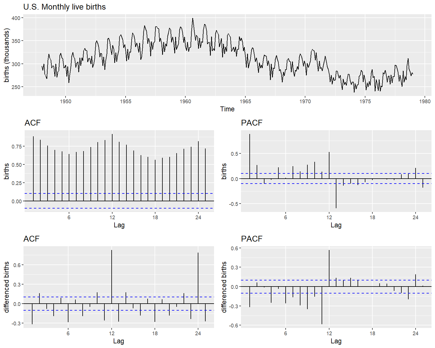
Monthly live birth U.S.A
For start, a multiplicative Seasonal ARIMA model could give a good fit to the data, following Tsay (2010) recommendations for order selection using the auto-correlation functions, we define (p = 1, d = 1, q = 1) and for the seasonal part (P= 1, D = 1 and Q = 1). The fitted model is defined as follows
sf1 = stan_sarima(ts = birth,order = c(1,1,1),seasonal = c(1,1,1),
                  prior_mu0 = student(mu = 0,sd = 1,df = 7))
All fitted models are varstan objects, these are S3 classes with the stanfit results provided by the rstan package, and other useful elements that make the modeling process easier.
sf1
#>
#> y ~ Sarima(1,1,1)(1,1,1)[12]
#> 373 observations and 1 dimension
#> Differences: 1 seasonal Differences: 1
#> Current observations: 360
#>
#>              mean     se         5%        95%      ess   Rhat
#> mu0        0.0017 0.0019    -0.1973     0.2014 3358.708 0.9998
#> sigma0     7.3412 0.0043     6.9097     7.8165 3951.632 0.9998
#> ar        -0.2522 0.0013    -0.3717    -0.1176 3985.357 1.0004
#> ma        -0.0336 0.0014    -0.1853     0.0818 3928.152 1.0009
#> sar        0.0086 0.0014    -0.1515     0.1425 3982.520 1.0008
#> sma       -0.6750 0.0015    -0.7887    -0.4982 3869.922 1.0004
#> loglik -1231.6717 0.0307 -1235.4485 -1229.2336 3867.011 1.0021
#>
#>  Samples were drawn using sampling(NUTS). For each parameter, ess
#>  is the effective sample size, and Rhat is the potential
#>  scale reduction factor on split chains (at convergence, Rhat = 1).
After fitting our model we can make a visual diagnostic of our parameters, check residuals and fitted values using the plot method. The package provides the posterior sample of every residual, but checking all of them is an exhausting task. An alternative, is checking the process generated by the residuals posterior estimate.
check_residuals(sf1)
A white noise behavior indicates a good model fit. The model’s residuals in figure 2, seems to follow a random noise, the auto-correlation in acf plots quickly falls to zero, indicating an acceptable model fit. Finally a forecast of the for the next year can be performed as:
autoplot(forecast(object = sf1,h = 12))
Automatic prediction is possible using the forecast function, by default the prediction is done using Generalized additive models from the prophet package.
library(astsa)
autoplot(object = forecast(cardox,h = 12),include = 100)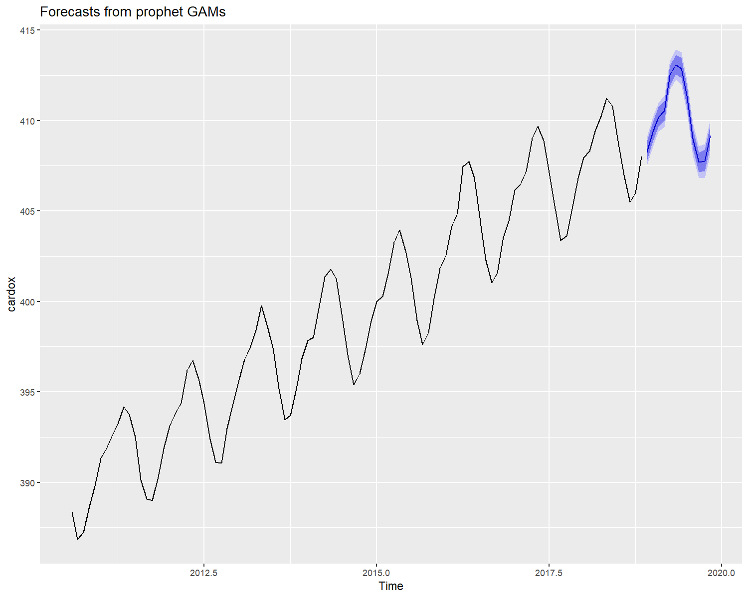
For further readings and references you can check:
Stan Development Team. 2018. Stan Modeling Language Users Guide and Reference Manual, Version 2.18.0. http://mc-stan.org
Forecasting: Principles and practice Monash University, Australia. Forecasting principles
Time Series Analysis and Its Applications, With R Examples — 4th Edition.astsa
facebook/prophet Quick start documentation. prophet
Orbit API Documentation and Examples. Orbit