![]()
pcsstools is an R package to describe various regression models using only pre-computed summary statistics (PCSS) from genome-wide association studies (GWASs) and PCSS repositories such as GeneAtlas. This eliminates the logistic, privacy, and access concerns that accompany the use of individual patient-level data (IPD).
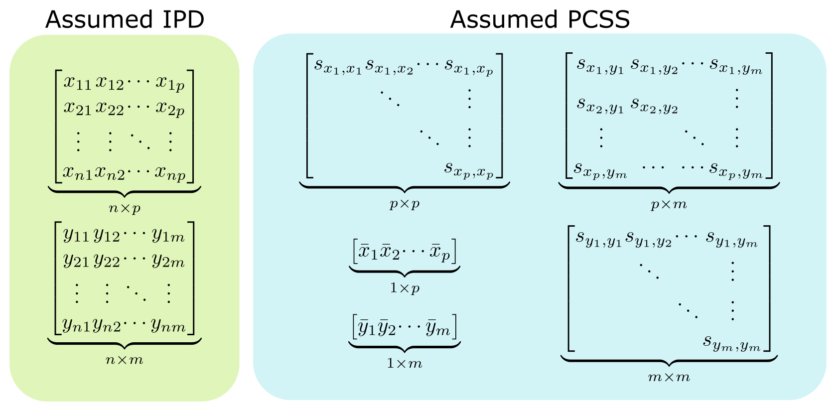
The following figure highlights the information typically needed to perform regression analysis on a set of m phenotypes with p covariates when IPD is available, and the PCSS that are commonly needed to approximate this same model in pcsstools.
Currently, pcsstools supports the linear modeling of complex phenotypes defined via functions of other phenotypes. Supported functions include:
You can install pcsstools from CRAN with
install.packages("pcsstools")You can install the in-development version of pcsstools from GitHub with
# install.packages("devtools")
devtools::install_github("jackmwolf/pcsstools")We will walk through two examples using pcsstools to model combinations of phenotypes using PCSS and then compare our results to those found using IPD.
library(pcsstools)Let’s model the first principal component score of three phenotypes using PCSS.
First, we’ll load in some data. We have three SNPs; minor allele
counts (g1, g2, and g3), a
continuous covariate (x1), and three continuous phenotypes
(y1, y2, and y3).
dat <- pcsstools_example[c("g1", "g2", "g3", "x1", "y1", "y2", "y3")]
head(dat)
#>   g1 g2 g3          x1         y1          y2          y3
#> 1  0  1  1  0.04239463 -0.1416907  1.19902689 -1.10982855
#> 2  1  0  0  1.35306987  0.6822496 -1.19624311 -0.97103574
#> 3  0  1  0 -1.01226388  0.8337136  0.75777722 -1.02609693
#> 4  0  1  0 -0.35358877 -0.1718187  1.13433957 -0.08290115
#> 5  1  1  0  1.20242824  0.5528258 -0.07515538 -2.43725278
#> 6  0  1  0  0.20310211 -0.9358902 -0.75434908 -1.59552034
First, we need our assumed summary statistics: means, the full covariance matrix, and our sample size.
pcss <- list(
  means = colMeans(dat),
  covs  = cov(dat),
  n     = nrow(dat)
)
Then, we can calculate the linear model by using
pcsslm(). Our formula will list all phenotypes
as one sum, joined together by + operators and we indicate
that we want the first principal component score by setting
comp = 1. We also want to center and standardize
y1, y2, and y3 before computing
principal component scores; we will do so by setting
center = TRUE and standardize = TRUE.
model_pcss <- pcsslm(y1 + y2 + y3 ~ g1 + g2 + g3 + x1, pcss = pcss, comp = 1,
                     center = TRUE, standardize = TRUE)
model_pcss
#> Model approximated using Pre-Computed Summary Statistics.
#>
#> Call:
#> pcsslm(formula = y1 + y2 + y3 ~ g1 + g2 + g3 + x1, pcss = pcss,
#>     comp = 1, center = TRUE, standardize = TRUE)
#>
#> Coefficients:
#>             Estimate Std. Error t value Pr(>|t|)
#> (Intercept) -0.03166    0.04710  -0.672 0.501581
#> g1           0.30333    0.04264   7.115 2.14e-12 ***
#> g2          -0.10125    0.03725  -2.718 0.006681 **
#> g3          -0.20014    0.05391  -3.713 0.000216 ***
#> x1           0.96190    0.02603  36.953  < 2e-16 ***
#> ---
#> Signif. codes:  0 '***' 0.001 '**' 0.01 '*' 0.05 '.' 0.1 ' ' 1
#>
#> Residual standard error: 0.8234 on 995 degrees of freedom
#> Multiple R-squared:  0.5891, Adjusted R-squared:  0.5874
#> F-statistic: 356.6 on 4 and 995 DF,  p-value: < 2.2e-16
Here’s the same model using individual patient data.
pc_1 <- prcomp(x = dat[c("y1", "y2", "y3")], center = TRUE, scale. = TRUE)$x[, "PC1"]

model_ipd <- lm(pc_1 ~ g1 + g2 + g3 + x1, data = dat)
summary(model_ipd)
#>
#> Call:
#> lm(formula = pc_1 ~ g1 + g2 + g3 + x1, data = dat)
#>
#> Residuals:
#>      Min       1Q   Median       3Q      Max
#> -2.48100 -0.55738 -0.00702  0.56556  2.42936
#>
#> Coefficients:
#>             Estimate Std. Error t value Pr(>|t|)
#> (Intercept)  0.03166    0.04710   0.672 0.501581
#> g1          -0.30333    0.04264  -7.115 2.14e-12 ***
#> g2           0.10125    0.03725   2.718 0.006681 **
#> g3           0.20014    0.05391   3.713 0.000216 ***
#> x1          -0.96190    0.02603 -36.953  < 2e-16 ***
#> ---
#> Signif. codes:  0 '***' 0.001 '**' 0.01 '*' 0.05 '.' 0.1 ' ' 1
#>
#> Residual standard error: 0.8234 on 995 degrees of freedom
#> Multiple R-squared:  0.5891, Adjusted R-squared:  0.5874
#> F-statistic: 356.6 on 4 and 995 DF,  p-value: < 2.2e-16
In this case, our coefficient estimates are off by a factor of -1;
this is because we picked the opposite vector of principal component
weights to prcomp. This distinction in sign is arbitrary
(see the note in ?prcomp).
We can also compare this model to a smaller model using
anova and find the same results when using both PCSS and
IPD.
model_pcss_reduced <- update(model_pcss, . ~ . - g1 - g2 - g3)
anova(model_pcss_reduced, model_pcss)
#> Analysis of Variance Table
#>
#> Model 1: y1 + y2 + y3 ~ x1
#> Model 2: y1 + y2 + y3 ~ g1 + g2 + g3 + x1
#>   Res.Df    RSS Df Sum of Sq      F    Pr(>F)
#> 1    998 723.16
#> 2    995 674.60  3    48.564 23.877 6.322e-15 ***
#> ---
#> Signif. codes:  0 '***' 0.001 '**' 0.01 '*' 0.05 '.' 0.1 ' ' 1

model_ipd_reduced <-update(model_ipd, . ~ . - g1 - g2 - g3)
anova(model_ipd_reduced, model_ipd)
#> Analysis of Variance Table
#>
#> Model 1: pc_1 ~ x1
#> Model 2: pc_1 ~ g1 + g2 + g3 + x1
#>   Res.Df    RSS Df Sum of Sq      F    Pr(>F)
#> 1    998 723.16
#> 2    995 674.60  3    48.564 23.877 6.322e-15 ***
#> ---
#> Signif. codes: 0 '***' 0.001 '**' 0.01 '*' 0.05 '.' 0.1 ' ' 1In this example we will approximate a linear model where our response is the logical combination “y4 or y5” (y4 ∨ y5).
First we need data with binary phenotypes.
dat <- pcsstools_example[c("g1", "g2", "x1", "y4", "y5")]
head(dat)
#>   g1 g2          x1 y4 y5
#> 1  0  1  0.04239463  1  0
#> 2  1  0  1.35306987  0  1
#> 3  0  1 -1.01226388  1  1
#> 4  0  1 -0.35358877  1  0
#> 5  1  1  1.20242824  0  0
#> 6  0  1  0.20310211  1  1
Once again we will organized our assumed PCSS. In addition to the
summary statistics we needed for the previous example, we also need to
describe the distributions of both of our predictors through objects of
class predictor. (See ?new_predictor.)
pcsstools has shortcut functions to create
predictor objects for common types of variables, which we
will use to create a list of predictors.
pcss <- list(
 means = colMeans(dat),
 covs = cov(dat),
 n = nrow(dat),
 predictors = list(
   g1 = new_predictor_snp(maf = mean(dat$g1) / 2),
   g2 = new_predictor_snp(maf = mean(dat$g2) / 2),
   x1 = new_predictor_normal(mean = mean(dat$x1), sd = sd(dat$x1))
 )
)

class(pcss$predictors[[1]])
#> [1] "predictor"
Then we can approximate the linear model using
pcsslm().
model_pcss <- pcsslm(y4 | y5 ~ g1 + g2 + x1, pcss = pcss)
model_pcss
#> Model approximated using Pre-Computed Summary Statistics.
#>
#> Call:
#> pcsslm(formula = y4 | y5 ~ g1 + g2 + x1, pcss = pcss)
#>
#> Coefficients:
#>             Estimate Std. Error t value Pr(>|t|)
#> (Intercept)  0.75383    0.01995  37.786  < 2e-16 ***
#> g1          -0.05257    0.01904  -2.761  0.00587 **
#> g2           0.11709    0.01664   7.038 3.62e-12 ***
#> x1          -0.08160    0.01163  -7.019 4.14e-12 ***
#> ---
#> Signif. codes:  0 '***' 0.001 '**' 0.01 '*' 0.05 '.' 0.1 ' ' 1
#>
#> Residual standard error: 0.3678 on 996 degrees of freedom
#> Multiple R-squared:  0.09521,    Adjusted R-squared:  0.09249
#> F-statistic: 34.94 on 3 and 996 DF,  p-value: < 2.2e-16
And here’s the result we would get using IPD:
model_ipd <- lm(y4 | y5 ~ g1 + g2 + x1, data = dat)
summary(model_ipd)
#>
#> Call:
#> lm(formula = y4 | y5 ~ g1 + g2 + x1, data = dat)
#>
#> Residuals:
#>      Min       1Q   Median       3Q      Max
#> -0.97250 -0.02297  0.12654  0.22802  0.54225
#>
#> Coefficients:
#>             Estimate Std. Error t value Pr(>|t|)
#> (Intercept)  0.74555    0.01970  37.849  < 2e-16 ***
#> g1          -0.06695    0.01880  -3.561 0.000387 ***
#> g2           0.13714    0.01643   8.349 2.28e-16 ***
#> x1          -0.08372    0.01148  -7.293 6.16e-13 ***
#> ---
#> Signif. codes:  0 '***' 0.001 '**' 0.01 '*' 0.05 '.' 0.1 ' ' 1
#>
#> Residual standard error: 0.3631 on 996 degrees of freedom
#> Multiple R-squared:  0.1179, Adjusted R-squared:  0.1153
#> F-statistic: 44.39 on 3 and 996 DF, p-value: < 2.2e-16Support function notation for linear combinations of phenotypes
(e.g. y1 - y2 + 0.5 * y3 ~ 1 + g + x) instead of requiring
a separate vector of weights
Support functions using . and - in the
dependent variable (e.g. y1 ~ .,
y1 ~ . -x)
Write a vignette
Following are the key references for the functions in this package
Wolf, J.M., Westra, J., and Tintle, N. (2021). Using summary statistics to model multiplicative combinations of initially analyzed phenotypes with a flexible choice of covariates. Frontiers in Genetics, 25, 1962. https://doi.org/10.3389/fgene.2021.745901.
Wolf, J.M., Barnard, M., Xueting, X., Ryder, N., Westra, J., and Tintle, N. (2020). Computationally efficient, exact, covariate-adjusted genetic principal component analysis by leveraging individual marker summary statistics from large biobanks. Pacific Symposium on Biocomputing, 25, 719-730. https://doi.org/10.1142/9789811215636_0063.
Gasdaska A., Friend D., Chen R., Westra J., Zawistowski M., Lindsey W. and Tintle N. (2019) Leveraging summary statistics to make inferences about complex phenotypes in large biobanks. Pacific Symposium on Biocomputing, 24, 391-402. https://doi.org/10.1142/9789813279827_0036.