![]()
![]()
A code-based reproducible package for generating representative points along road networks within regions–“pseudohouseholds”–that can be used for population-weighted travel analyses.
You can install the current published version of pseudohouseholds from CRAN with:
install.packages("pseudohouseholds")You can install the development version of pseudohouseholds from GitHub with:
# install.packages("devtools")
devtools::install_github("chris31415926535/pseudohouseholds")This vignette provides an overview of what pseudohouseholds (PHHs) are, and how you can use the pseudohouseholds package to help create them.
In brief, PHHs are representative points placed along road segments and inside regions that provide spatial distributions of some region-specific property (in practice, usually population). They provide an approximate way of “spreading out” regional population distributions that can be helpful when doing travel analyses. We say that PHHs are “pseudo” households because they do not represent actual buildings or households, but they approximate the distribution of households by creating a set of populated points where we think the households are likely to be. This can allow us to create finer-grained travel or coverage analyses.
By contrast, many travel analyses assume that a region’s entire population is concentrated at a single point, usually the region’s centroid. While this assumption can be valid for smaller regions like city blocks, it breaks in larger or rural regions where the population may be more dispersed, or regions with unusual shapes that may not contain their own centroids.
Let’s walk through the algorithm by giving a demonstration using test data included with the package. We’ll consider a single dissemination block (DB) in Ottawa, Ontario, with unique identifier (DBUID) “35061699003”. DBs are the smallest region at which Statistics Canada makes population data available, so they’re a good starting point for a fine-grained analysis.
Here we load our packages, isolate our DB, and print it to the console:
library(sf)
#> Linking to GEOS 3.10.2, GDAL 3.4.1, PROJ 8.2.1; sf_use_s2() is TRUE
library(ggplot2)
library(ggspatial)
library(pseudohouseholds)

db <- dplyr::filter(pseudohouseholds::ottawa_db_shp, DBUID == "35061699003")

print(db)
#> Simple feature collection with 1 feature and 2 fields
#> Geometry type: MULTIPOLYGON
#> Dimension:     XY
#> Bounding box:  xmin: 369747.8 ymin: 5027016 xmax: 370185.7 ymax: 5027330
#> Projected CRS: NAD83 / MTM zone 9
#> # A tibble: 1 × 3
#>   DBUID       dbpop2021                                                 geometry
#> * <chr>           <dbl>                                       <MULTIPOLYGON [m]>
#> 1 35061699003       125 (((370113.7 5027251, 370075.7 5027241, 370026.3 5027236…
Note that its coordinate reference system (CRS) is projected. Specifically, it’s using NAD83/MTM zone 9 (32189) which gives units in meters. It’s important to use a projected CRS with this package.
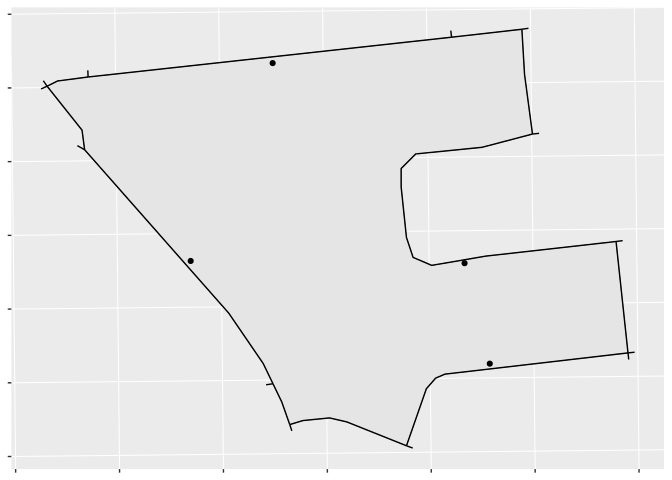
Let’s also plot it to get an idea of its scale:
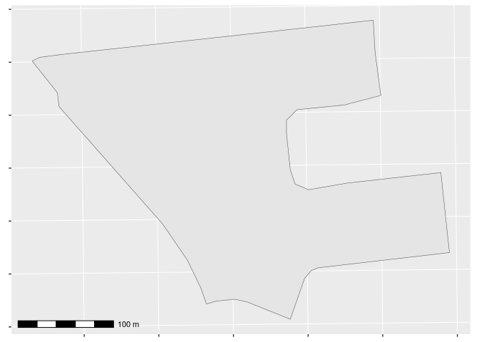
This DB is a few hundred meters across, borders Bank St. on its west, and extends to the east into an irregularly shaped residential area. From the printout above, we see that it had a population of 125 in 2021.
By default, if a region is unpopulated it receives one single point
with population 0 of phh_type type 1. This point will be
the centroid if it is inside the region, otherwise it will be an
approximation of the region’s “pole of inaccessibility.” Details are
provided below.
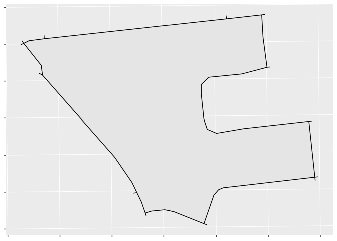
First, we identify road segments that either intersect with the region or come within a specified buffer. The default buffer is 5 meters, which we adopt here, although larger or smaller buffers may be appropriate in different settings.
Plotting our DB and the road segments that intersect it:
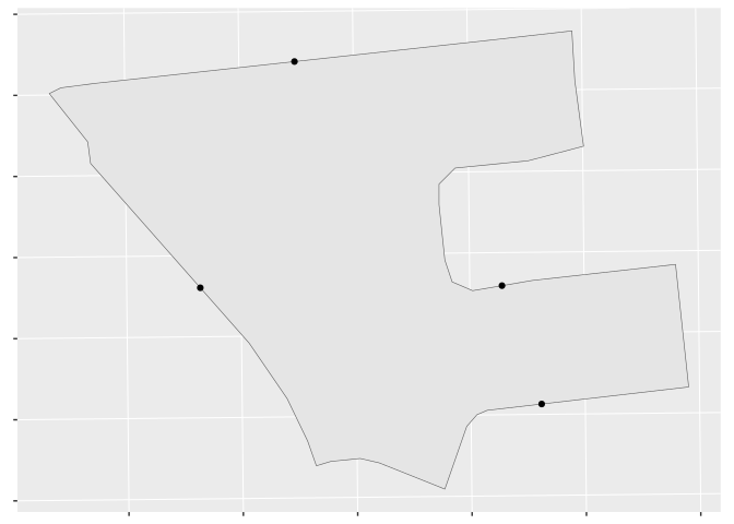
Next we sample points along these road segments. The sampling
frequency is given by the parameter phh_density, which is
passed along directly to the function sf::st_line_sample()
and is measured in units of “PHHs per unit.” The default value is 0.005
which, in meters, translates to one PHH every 200 meters. Note that this
is for our initial sampling, and that the final PHHs may be closer or
farther than this.
Optionally, users can set a desired minimum number of regional PHHs
using the parameter min_phhs_per_region, which can be
helpful with smaller regions (e.g. small city blocks).
We want our PHHs to be inside our DB, so our next step is to
perturb these points by the distance delta_distance to try
to create candidates within the region. To do so, we:
delta_distance; and,delta_distance.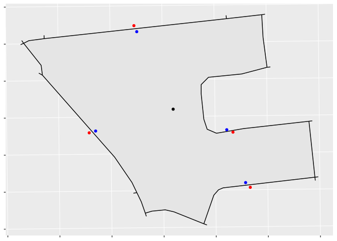
As can be seen, most of the blue “pull” candidates are within the DB and most of the “push” candidates are outside; however, because of the DB’s odd geometry, one “pull” candidate is outside, and one “push” is inside. Creating two sets of candidates increases the algorithm’s processing overhead, but it helps to ensure that our PHHs are distributed the way we want.
Next, we keep only those candidate PHHs that are inside the region using a spatial filter.
The push/pull algorithm may not return valid PHHs in some cases, for
example if the region is concave and has only small intersections with
any road. In this case we use a backup algorithm that samples 16
candidate points distributed radially with radius
delta_distance around our on-street point and selects the
first candidate point within the region.
If for any reason the algorithm has still not found a valid candidate
PHH, it will now return a single default point. It will return the
centroid if the centroid is inside the region, or else an approximation
of the visual centre of the region. In either case this point will have
phh_type 2, indicating no valid PHHs were found using the
standard methods.
If we are assigning populations to our PHHs, we next check to ensure
each PHH will have at least some minimum population set by the parameter
min_phh_pop. This is helpful for “thinning out” PHHs in
large sparsely-populated rural areas, where the default line sampling
density would lead to a large number of PHHs with populations less than
1.
This can be disabled by setting min_phh_pop to 0.
Optionally, we can remove any PHHs that are within
min_phh_distance units of another. This is helpful to
reduce artificial over-crowding caused by specific road features: for
example, if many short road segments converge, each could receive a
candidate PHH from sf::st_line_sample().
We now have a set of points that are near a road, within the region, and not too close together. The final step is to assign each PHH an equal share of the region’s population.
The algorithm attempts to satisfy several competing criteria–the
minimum number of PHHs per region, the minimum population of those PHHs,
and the minimum distance between them–and it may not be possible to meet
them all. In particular, it will make its best effort to satisfy
min_phhs_per_region, but min_phh_pop and
min_phh_distance take precedence.
Standard GIGO principles apply, so if there are any roads where you don’t want PHHs (e.g. highways, service roads, unpaved trails), take care to remove them beforehand.
Any analysis using PHHs should be clear that they rely on approximations and do not provide “true” population distributions (whatever that might even mean). While PHHs can provide advantages over centroid-based analyses, they also have limitations and should be used with these limitations in mind.
phh_typeIf a region is unpopulated or if it is no valid PHHs can be found, the function will return the region’s “default point.” If the region’s centroid is inside it, the default point is the centroid. If the centroid is outside the region, we use a simple algorithm to choose a point that is approximately in the region’s “pole of inaccessibility,” or farthest from each border: we randomly sample 100 points inside the region, and choose the one that is farthest from any border.
Such points are flagged as either phh_type 1
(unpopulated) or phh_type 2 (populated but no valid PHHs
found), and care should be taken when using these variables for analysis
since they may be farther from road networks than regular PHHs and may
not represent actual population distributions.