TWO-SIGMA:
Van Buren, E, Hu, M, Weng, C, et al. TWO‐SIGMA: A novel two‐component single cell model‐based association method for single‐cell RNA‐seq data. Genetic Epidemiology. 2020; 1– 12. https://doi.org/10.1002/gepi.22361
TWO-SIGMA-G bioRxiv preprint:
TWO-SIGMA-G: A New Competitive Gene Set Testing Framework for scRNA-seq Data Accounting for Inter-Gene and Cell-Cell Correlation: doi: https://doi.org/10.1101/2021.01.24.427979
Eric Van Buren: evb@hsph.harvard.edu, Di Wu: did@email.unc.edu, Yun Li: yun_li@med.unc.edu
twosigma is an R package for differential expression
(DE) analysis and DE-based gene set testing (GST) in single-cell RNA-seq
(scRNA-seq) data. At the gene-level, DE can be assessed by fitting our
proposed TWO-component SInGle cell Model-based Association method
(TWO-SIGMA). The first component models the drop-out probability with a
mixed effects logistic regression, and the second component models the
(conditional) mean read count with a mixed-effects log-linear negative
binomial regression. Our approach thus allows for both excess zero
counts and overdispersed counts while also accommodating dependency in
both drop-out probability and mean mRNA abundance. TWO-SIGMA is
especially useful in its flexibility to analyze DE beyond a two-group
comparison while simultaneously controlling for additional subject-level
or cell-level covariates including batch effects. At the set-level, the
package can perform competitive DE-based gene set testing using our
proposed TWO-SIGMA-G method. Users can specify the number of cores to be
used for parallelization in all functions using the ncores argument.
We recommend installing from GitHub or CRAN for the latest version (1.0.2) of the package, which is built for any version of R >= 3.6.3 (including R >= 4.0):
install.packages("twosigma")
# OR
install.packages("devtools")
devtools::install_github("edvanburen/twosigma")

library(twosigma)
Note the following minimum package versions for imported packages:
multcomp (>= 1.4-13), methods, pscl (>= 1.5.5), pbapply (>=
1.4.0), parallel (>= 3.6.3), doParallel (>= 1.0.15). ## Gene-Level
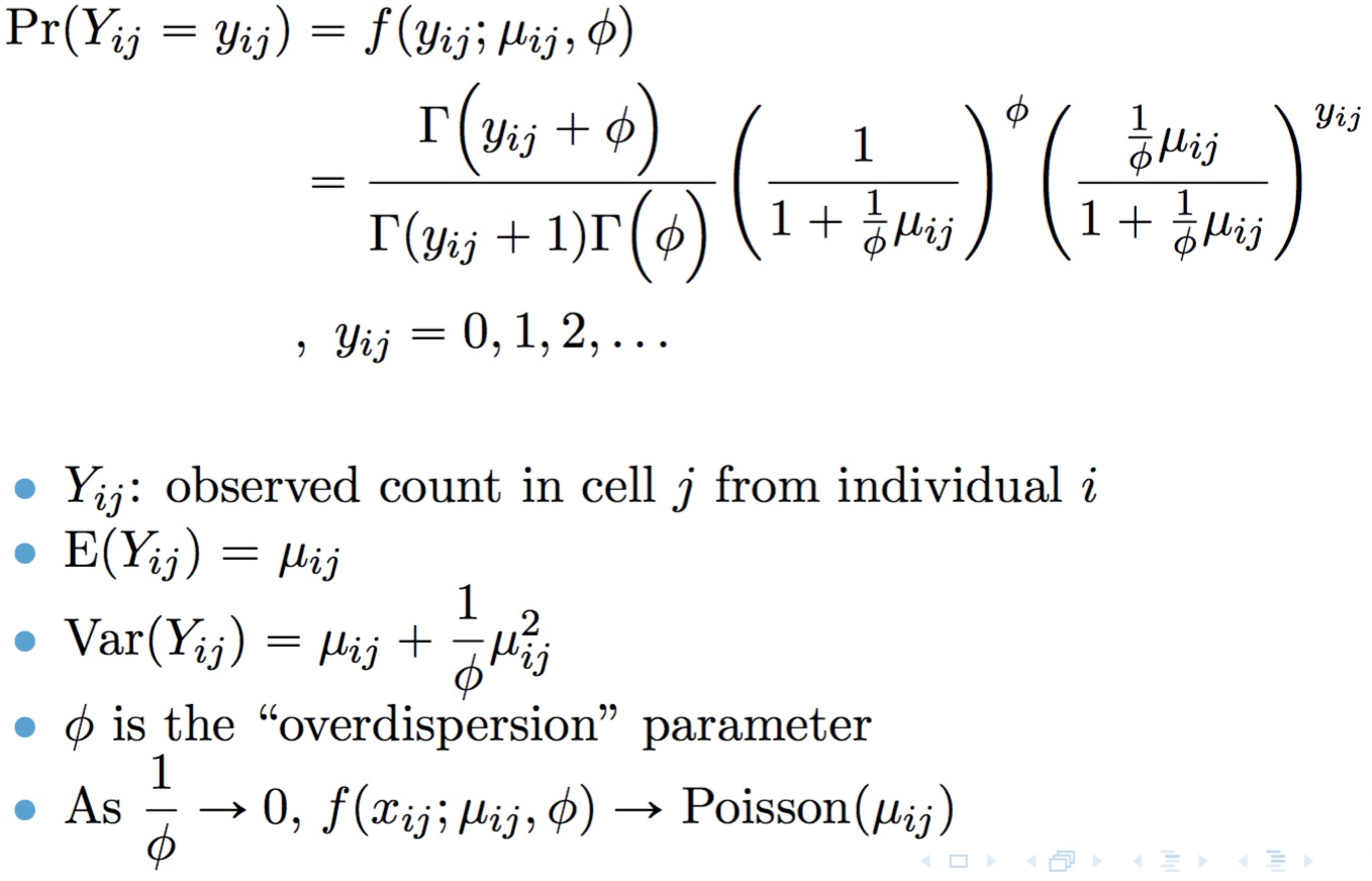
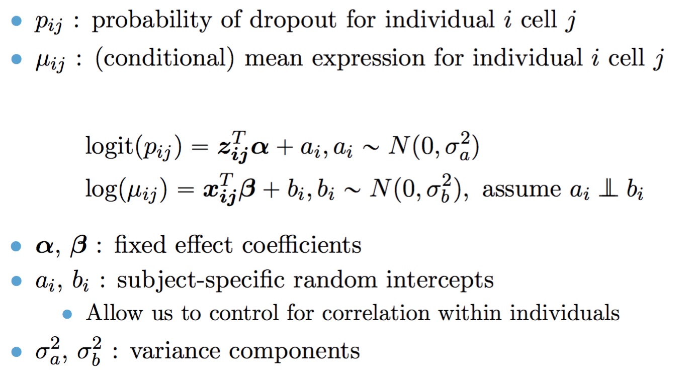
Model TWO-SIGMA is based on the following parameterization of the
negative binomial distribution:
A point mass at zero is added to the distribution to account for dropout. The result is the probability mass function for the zero-inflated negative binomial distribution:
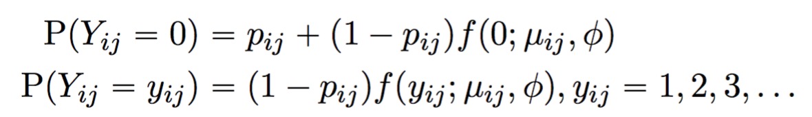
The full TWO-SIGMA specification is therefore as follows:
The workhorse function is twosigma, which can be easiest called as
twosigma(count_matrix, mean_covar, zi_covar,id,ncores=1)By default, we employ our ad hoc procedure to determine if random effects are needed. If users wish to specify their own random effect specifications, they can set adhoc=FALSE, and use the following inputs:
If adhoc=TRUE, mean_re and zi_re are ignored and a
warning is printed.
If users wish to customize the random effect or fixed effect
specification, they may do so via the function twosigma_custom
, which has the following basic syntax:
twosigma_custom(count_matrix, mean_form, zi_form, id) mean_form = count ~ 1 ~ 1
Some care must be taken, however, because these formulas are used
directly. It is therefore the user’s responsibility to ensure
that formulas being inputted will operate as expected. Syntax
is identical to the lme4 package.
For example, each of the following function calls reproduces the default TWO-SIGMA specification with random intercepts in both components:
fits<-twosigma(count_matrix, mean_covar=mean_covar_matrix, zi_covar=zi_covar_matrix, mean_re = TRUE, zi_re = TRUE, id=id,adhoc=F)
fits2<-twosigma_custom(count, mean_form=count~mean_covar_matrix+(1|id),zi_form=~zi_covar_matrix+(1|id),id=id)If users wish to jointly test a fixed effect using the twosigma model
via the likelihood ratio test, they may do so using the
lr.twosigma or lr.twosigma_custom functions:
lr.twosigma(count_matrix, mean_covar, zi_covar, covar_to_test, mean_re = TRUE,zi_re = TRUE, disp_covar = NULL,adhoc=TRUE)
lr.twosigma_custom(count_matrix, mean_form_alt, zi_form_alt, mean_form_null, zi_form_null, id, lr.df)The lr.twosigma function assumes that the variable being
tested is in both components of the model (and thus that the
zero-inflation component exists and contains more than an Intercept).
Users wishing to do fixed effect testing in other cases can use the
lr.twosigma_custom function with custom formulas or
construct the test themselves using two calls to twosigma
twosigma_custom. The formula inputs mean_form_alt
, mean_form_null, zi_form_alt, and
zi_form_null should be specified as in the
lr.twosigma_custom function and once again users must
ensure custom formulas represent a valid likelihood ratio test.
One part of this responsibility is specifying the argument
lr.df giving the degrees of freedom of the likelihood ratio
test.
Assume fits is an object returned from
twosigma or twosigma_custom. Then, we can get
some gene-level information using:
calc_logFC<-function(x){
    if(class(x)=="glmmTMB"){x<-summary(x)}
    if(is.character(x)){return(NA)}else{
      x$coefficients$cond['t2d_sim','Estimate']
    }
}
calc_Z<-function(x){
    if(class(x)=="glmmTMB"){x<-summary(x)}
    if(is.character(x)){return(NA)}else{
      x$coefficients$cond['t2d_sim','z value']
    }
}
calc_p.vals<-function(x){
    if(class(x)=="glmmTMB"){x<-summary(x)}
    if(is.character(x)){return(NA)}else{
      x$coefficients$cond['t2d_sim',4]
    }
}
calc_Stouffer<-function(x){
    if(class(x)=="glmmTMB"){x<-summary(x)}
    if(is.character(x)){return(NA)}else{
      (x$coefficients$cond['t2d_sim','z value']+x$coefficients$cond['t2d_sim','z value'])/sqrt(2)
    }
}

logFC<-unlist(lapply(fits$fit,calc_logFC))
Zstats<-unlist(lapply(fits$fit,calc_Z))
p.val_Zstat<-unlist(lapply(fits$fit,calc_p.vals)
Stouffer<-unlist(lapply(fits$fit,calc_Stouffer))Functionality to do this is ongoing. For now, individuals can use the
twosigmag function for TWO-SIGMA based Gene-Set Testing to
test custom contrast matrices (even if not interested in gene set
testing, simply set index_test=list(c(1,2)) and
all_as_ref=TRUE and look at gene-level output).
As mentioned in the paper, we mention a method that can be useful in selecting genes that may benefit from the inclusion of random effect terms. This method fits a zero-inflated negative binomial model without random effects and uses a one-way ANOVA regressing the Pearson residuals on the individual ID to look for differences between individuals.
adhoc.twosigma(count, mean_covar, zi_covar, id)The p-value from the ANOVA F test is returned, and can be used as a
screening for genes that are most in need of random effects. This
functionality is built into the twosigma function so
users likely do not need to call directly themselves.
As discussed in the main text, one can use the likelihood ratio test
to test either one or both components for random effect terms via the
function test.vc.twosigma Which components contain random
effects under the alternative are controlled by mean_re and
zi_re.
Competitive gene set testing based on TWO-SIGMA can be performed
using the function twosigmag. Gene-level statistics
currently implemented include likelihood ratio, Z-statistic from the
mean model, Stouffer’s combination of the Z-statistics from the mean and
ZI model, or a test of a custom contrast matrix. If a contrast matrix is
input, set-level results are returned for each row of the contrast.
Multiple cores are once again recommended if possible,
particularly if using the likelihood ratio test.
The adhoc procedure is not recommended for use in gene set testing. This is because geneset testing relies on a common gene-level null hypothesis being tested. When some genes have random effects and others do not, it is not clear that this requirement is met. Arguments which require more explanation over above are given as follows:
Multiple cores are once again recommended if possible, particularly if using the likelihood ratio test.
#--------------------------------------------------
#--- Simulate Data
#--------------------------------------------------

#Set parameters for the simulation
# This is as was done in the TWO-SIGMA paper
set.seed(1234)
nind<-10
ncellsper<-rep(1000,nind)
sigma.a<-.1
sigma.b<-.1
alpha<-c(-1,0,-.5,-2)
beta<-c(2,0,-.1,.6)
phi<-.1
id.levels<-1:nind


# Simulate some covariates
t2d_ind<-rbinom(nind,1,p=.4)
t2d_sim<-rep(t2d_ind,times=ncellsper)
nind<-length(id.levels)
id<-rep(id.levels,times=ncellsper)
cdr_sim<-rbeta(sum(ncellsper),3,6)
age_sim_ind<-sample(c(20:60),size=nind,replace = TRUE)
age_sim<-rep(age_sim_ind,times=ncellsper)

#Construct design matrices
Z<-cbind(t2d_sim,age_sim,cdr_sim)
colnames(Z)<-c("t2d_sim","age_sim","cdr_sim")
X<-cbind(t2d_sim,age_sim,cdr_sim)
colnames(X)<-c("t2d_sim","age_sim","cdr_sim")

sim_dat<-simulate_zero_inflated_nb_random_effect_data(ncellsper,X,Z,alpha,beta,phi,sigma.a,sigma.b,
                                                      id.levels=NULL)
sim_dat2<-simulate_zero_inflated_nb_random_effect_data(ncellsper,X,Z,alpha,beta,phi,sigma.a,sigma.b,
                                                      id.levels=NULL)

#--------------------------------------------------
#--- Fit TWO-SIGMA to simulated data
#--------------------------------------------------
id<-sim_dat$id

#matrix input required
counts<-matrix(rbind(sim_dat$Y,sim_dat2$Y),nrow=2,byrow=FALSE)
rownames(counts)<-paste0("Gene ",1:2)

fit<-twosigma(counts,zi_covar=Z,mean_covar = X,id=id,mean_re=FALSE,zi_re=FALSE,adhoc=F,ncores=1)
fit2<-twosigma_custom(counts, mean_form=count~t2d_sim+age_sim+cdr_sim
                      ,zi_form=~t2d_sim+age_sim+cdr_sim,id=id,ncores=1)

#fit and fit2 are the same for the both genes

fit$fit[[1]];fit2$fit[[1]]
fit$fit['Gene 2'];fit2$fit['Gene 2']

#--- Fit TWO-SIGMA without a zero-inflation component
fit_noZI<-twosigma(counts,zi_covar=0,mean_covar = X,id=id,mean_re=F,zi_re=F,adhoc=F,ncores=1)
fit_noZ2I<-twosigma_custom(counts,zi_form=~0,mean_form=count~X,id=id,ncores=1)

#--- Fit TWO-SIGMA with an intercept only zero-inflation component and no random effects
fit_meanZI<-twosigma(counts,zi_covar=1,mean_covar = X,id=id,mean_re=F,zi_re=F,adhoc=F,ncores=1)
fit_meanZI2<-twosigma_custom(counts, mean_form=count~t2d_sim+age_sim+cdr_sim,zi_form=~1,id=id,ncores=1)

fit_noZI$fit[['Gene 1']]
fit_meanZI$fit[['Gene 1']]

# Perform Likelihood Ratio Test on variable "t2d_sim"

lr.fit<-lr.twosigma(counts,covar_to_test="t2d_sim",mean_covar = X,zi_covar=Z,id=id)
lr.fit$LR_stat
lr.fit$LR_p.val

# Same results using lr.twosigma_custom

lr.fit_custom<-lr.twosigma_custom(counts,mean_form_alt=count~t2d_sim+age_sim+cdr_sim
, zi_form_alt=~t2d_sim+age_sim+cdr_sim, mean_form_null=count~age_sim+cdr_sim
,zi_form_null=~age_sim+cdr_sim,id=id,lr.df=2)

lr.fit_custom$LR_stat
lr.fit_custom$LR_p.val

#--------------------------------------------------
# Perform Gene-Set Testing
#--------------------------------------------------

# First, simulate some DE genes and some non-DE genes
set.seed(123)
sim_dat2<-matrix(nrow=10,ncol=sum(ncellsper))
beta<-c(2,0,-.1,.6)
beta2<-c(2,.5,-.1,.6)
for(i in 1:nrow(sim_dat2)){
  if(i<5){
    sim_dat2[i,]<-simulate_zero_inflated_nb_random_effect_data(ncellsper,X,Z,alpha,beta2,phi,sigma.a,sigma.b=.5,
      id.levels=NULL)$Y
  }else{
    sim_dat2[i,]<-simulate_zero_inflated_nb_random_effect_data(ncellsper,X,Z,alpha,beta,phi,sigma.a,sigma.b,
      id.levels=NULL)$Y
  }
}

# Use Z-statistic

gst2<-twosigmag(sim_dat2,index_test = list("Set 1" = c(6:10),"Set 2" = c(1:5)),mean_form = count~t2d_sim+age_sim+cdr_sim
,zi_form = ~t2d_sim+age_sim+cdr_sim,id=id,covar_to_test  = "t2d_sim"
,statistic = "Z",ncores=1)

gst2$set_p.val

# Testing a simple contrast equivalent to the Z statistic for 't2d_sim'

gst3<-twosigmag(sim_dat2,index_test = list("Set 1" = c(6:10),"Set 2" = c(1:5)),mean_form = count~t2d_sim+age_sim+cdr_sim
,zi_form = ~t2d_sim+age_sim+cdr_sim,id=id,statistic = "contrast"
,contrast_matrix = matrix(c(0,1,0,0),nrow=1),ncores = 1)

# Same result as using Z test

gst3$set_p.val
gst2$set_p.val


# Testing a contrast of a factor variable
# set seed to make sure factor has all three levels
# so contrast matrix is properly defined
set.seed(1234)
fact<-factor(rep(sample(c(0,1,2),nind,replace=T),times=ncellsper))
cont_matrix<-matrix(c(-1,1,0,-1,0,1),nrow=2,byrow = T)
rownames(cont_matrix)<-c("Test 1","Test 2")

gst4<-twosigmag(sim_dat2,index_test = list("Set 1" = c(6:10),"Set 2" = c(1:5))
,mean_form = count~t2d_sim+age_sim+cdr_sim+fact
,zi_form = ~t2d_sim+age_sim+cdr_sim,id=rep(id.levels,times=ncellsper)
,statistic = "contrast",contrast_matrix = cont_matrix
  ,factor_name="fact",ncores = 1,return_summary_fits = T)

# Finally, test the factor "manually"" to show results are the same
cont_matrix2<-matrix(c(0,0,0,0,1,0,0,0,0,0,0,1),nrow=2,byrow = T)
rownames(cont_matrix2)<-c("Test 1","Test 2")

gst5<-twosigmag(sim_dat2,index_test = list("Set 1" = c(6:10),"Set 2" = c(1:5)),mean_form = count~t2d_sim+age_sim+cdr_sim+fact
,zi_form = ~t2d_sim+age_sim+cdr_sim,id=id,statistic = "contrast",contrast_matrix = cont_matrix2
,ncores = 1,return_summary_fits = T)

#Two give the same results

gst4$set_p.val
gst5$set_p.val

gst6<-twosigmag(sim_dat2,index_test = list("Set 1" = c(6:10),"Set 2" = c(1:5)),mean_form = count~t2d_sim+age_sim+cdr_sim+fact
,zi_form = ~t2d_sim+age_sim+cdr_sim,id=id,statistic = "contrast",contrast_matrix = cont_matrix2
,ncores = 1,return_summary_fits = T)


#Plot Results in Heatmaps
library(pheatmap)
plot_tsg<-function(obj,top_set_size_ct=10,font_size=10,set_cex=.7,plot_title="Title"){
    j<-0
    for(i in colnames(obj$set_p.val)){
      j<-j+1
      assign(paste0(i,"_topsets"),rownames(obj$estimates_set_level)[order(obj$estimates_set_level[,i],decreasing = F)][1:top_set_size_ct])
    }
    all_sets<-sort(unique(c(sapply(ls(pattern="topsets"),FUN = get,envir=sys.frame(sys.parent(0))))))
    # Put Sets in Order of significance in top cell type
    mat_plot<-obj$estimates_set_level[all_sets,]
    colors<-colorRampPalette(c('blue',"white", 'red'))(13)
    plot_colors<-c(colors[1:5],"#FFFFFF","#FFFFFF",colors[8:13])

    b<-pheatmap(as.matrix(t(mat_plot)),fontsize=font_size,fontsize_col = set_cex*font_size,main = plot_title,breaks=c(-.5,-.4,-.3,-.2,-.1,-.001,0,.001,.1,.2,.3,.4,.5),border_color = NA,na_col='grey',cellwidth = 10,cellheight=30,color=plot_colors)
    #left to right
    set_order2<-b$tree_col$order
    # bottom to top
    ct_order2<-b$tree_row$order
    mat_plot<-obj$set_p.val[all_sets,]
    mat_plot<-log10(mat_plot)
    mat_plot<-mat_plot[set_order2,ct_order2]
    pheatmap(mat=as.matrix(t(mat_plot)),cluster_rows=FALSE,main = "Heatmap of Set-Level log10 p-values (Unadjusted) by Cell Type",cellwidth = 10,cellheight=30,show_colnames = T,
             cluster_cols=FALSE,fontsize=font_size,fontsize_col = set_cex*font_size,border_color = NA
             ,na_col='grey',color=colorRampPalette(c('darkgreen',"white"))(12))

  }

plot_tsg(gst6)