

The goal of GGMnonreg is to estimate non-regularized graphical models. Note that the title is a bit of a misnomer, in that Ising and mixed graphical models are also supported.
Graphical modeling is quite common in fields with wide data, that is, when there are more variables than observations. Accordingly, many regularization-based approaches have been developed for those kinds of data. There are key drawbacks of regularization when the goal is inference, including, but not limited to, the fact that obtaining a valid measure of parameter uncertainty is very (very) difficult.
More recently, graphical modeling has emerged in psychology (Epskamp et al. 2018), where the data is typically long or low-dimensional (p < n; Donald R. Williams et al. 2019; Donald R. Williams and Rast 2019). The primary purpose of GGMnonreg is to provide methods specifically for low-dimensional data (e.g., those common to psychopathology networks).
The following are also included
You can install the development version from GitHub with:
# install.packages("devtools")
devtools::install_github("donaldRwilliams/GGMnonreg")An Ising model is fitted with the following
library(GGMnonreg)

# make binary
Y <- ifelse(ptsd[,1:5] == 0, 0, 1)

# fit model
fit <- ising_search(Y, IC = "BIC",
                    progress = FALSE)

fit
#>          1        2        3        4        5
#> 1 0.000000 1.439583 0.000000 1.273379 0.000000
#> 2 1.439583 0.000000 1.616511 0.000000 1.182281
#> 3 0.000000 1.616511 0.000000 1.716747 1.077322
#> 4 1.273379 0.000000 1.716747 0.000000 1.662550
#> 5 0.000000 1.182281 1.077322 1.662550 0.000000
Note the same code, more or less, is also used for GGMs and mixed graphical models.
It is common to compute predictability, or variance explained, for each node in the network. An advantage of GGMnonreg is that a measure of uncertainty is also provided.
# data
Y <- na.omit(bfi[,1:5])

# fit model
fit <- ggm_inference(Y, boot = FALSE)

# predictability
predictability(fit)
#>   Estimate Est.Error Ci.lb Ci.ub
#> 1     0.13      0.01  0.11  0.15
#> 2     0.33      0.01  0.30  0.36
#> 3     0.38      0.01  0.35  0.41
#> 4     0.18      0.01  0.15  0.20
#> 5 0.29 0.01 0.26 0.32Confidence intervals for each relation are obtained with
# data
Y <- na.omit(bfi[,1:5])

# fit model
fit <- ggm_inference(Y, boot = TRUE,
                     method = "spearman",
                     B = 100, progress = FALSE)

confint(fit)
#>              2.5%       97.5%
#>  [1,] -0.28754928 -0.22133409
#>  [2,] -0.14814197 -0.07708535
#>  [3,]  0.25745801  0.32050965
#>  [4,] -0.04829816  0.02726491
#>  [5,]  0.12384106  0.19379349
#>  [6,]  0.13688030  0.20747812
#>  [7,] -0.06140196  0.01178691
#>  [8,]  0.11399009  0.19706111
#>  [9,]  0.33858068  0.41127422
#> [10,]  0.08526116  0.15219698
These can then be plotted with, say, ggplot2 (left to the user).
When mining data, or performing an automatic search, it is difficult to make inference on the network parameters (e.g., confidence are not easily computed). To summarize data mining, GGMnonreg provides edge inclusion “probabilities” (proportion bootstrap samples for which each relation was detected).
# data
Y <- na.omit(bfi[,1:5])

# fit model
fit <-  eip(Y, method = "spearman",
            B  = 100, progress = FALSE)

fit
#>     eip
#> 1  1.00
#> 2  1.00
#> 3  1.00
#> 4  0.03
#> 5  1.00
#> 6  1.00
#> 7  0.35
#> 8  1.00
#> 9  1.00
#> 10 1.00
Note in all cases, the provided estimates correspond to the upper-triangular elements of the network.
GGMnonreg allows for computing expected network replicability (ENR), i.e., the number of effects that will be detected in any number of replications. This is an analytic solution.
The first step is defining a true network
# first make the true network
cors <- cor(GGMnonreg::ptsd)

# inverse
inv <- solve(cors)

# partials
pcors <-  -cov2cor(inv)

# set values to zero
pcors <- ifelse(abs(pcors) < 0.05, 0, pcors)
Then obtain ENR
fit_enr <- enr(net = pcors, n = 500, replications = 2)

fit_enr
#> Average Replicability: 0.45
#> Average Number of Edges: 53 (SD = 3.7)
#>
#> ----
#>
#> Cumulative Probability:
#>
#>  prop.edges edges Pr(R > prop.edges)
#>         0.0     0               1.00
#>         0.1    12               1.00
#>         0.2    23               1.00
#>         0.3    35               1.00
#>         0.4    47               0.91
#>         0.5    58               0.05
#>         0.6    70               0.00
#>         0.7    82               0.00
#>         0.8    94               0.00
#>         0.9   105               0.00
#> ----
#> Pr(R > prop.edges):
#> probability of replicating more than the
#> correpsonding proportion (and number) of edges
Note this is inherently frequentist. As such, over the long run, 45 % of the edges will be replicated on average. Then we can further infer that, in hypothetical replication attempts, more than half of the edges will be replicated only 5 % of the time.
ENR can also be plotted
plot(fit_enr)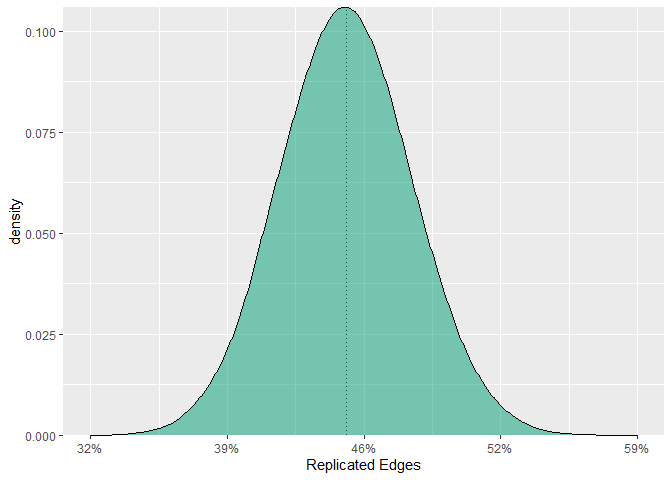
Here is the basic idea of ENR
# location of edges
index <- which(pcors[upper.tri(diag(20))] != 0)

# convert network into correlation matrix
diag(pcors) <- 1
cors_new <- corpcor::pcor2cor(pcors)

# replicated edges
R <- NA

# increase 1000 to, say, 5,000
for(i in 1:1000){

  # two replications
  Y1 <- MASS::mvrnorm(500, rep(0, 20), cors_new)
  Y2 <- MASS::mvrnorm(500, rep(0, 20), cors_new)

  # estimate network 1
  fit1 <- ggm_inference(Y1, boot = FALSE)

  # estimate network 2
  fit2 <- ggm_inference(Y2, boot = FALSE)

  # number of replicated edges (detected in both networks)
  R[i] <- sum(
    rowSums(
      cbind(fit1$adj[upper.tri(diag(20))][index],
            fit2$adj[upper.tri(diag(20))][index])
    ) == 2)
}
Notice that replication of two networks is being assessed over the long run. In other words, if we draw two random samples, what is the expected replicability.
Compare analytic to simulation
# combine simulation and analytic
cbind.data.frame(
  data.frame(simulation = sapply(seq(0, 0.9, 0.1), function(x) {
    mean(R > round(length(index) * x) )
  })),
  data.frame(analytic = round(fit_enr$cdf, 3))
)
#>    simulation analytic
#> 1       1.000    1.000
#> 2       1.000    1.000
#> 3       1.000    1.000
#> 4       1.000    1.000
#> 5       0.898    0.912
#> 6       0.044    0.052
#> 7       0.000    0.000
#> 8       0.000    0.000
#> 9       0.000    0.000
#> 10      0.000    0.000

# average replicability (simulation)
mean(R / length(index))
#> [1] 0.4468462

# average replicability (analytic)
fit_enr$ave_pwr
#> [1] 0.4485122
ENR works with any correlation, assuming there is an estimate of the standard error.
# data
Y <- ptsd

# estimate graph
fit <- ggm_inference(Y, boot = FALSE)

# get info for plotting
plot(get_graph(fit), edge_magnify = 5)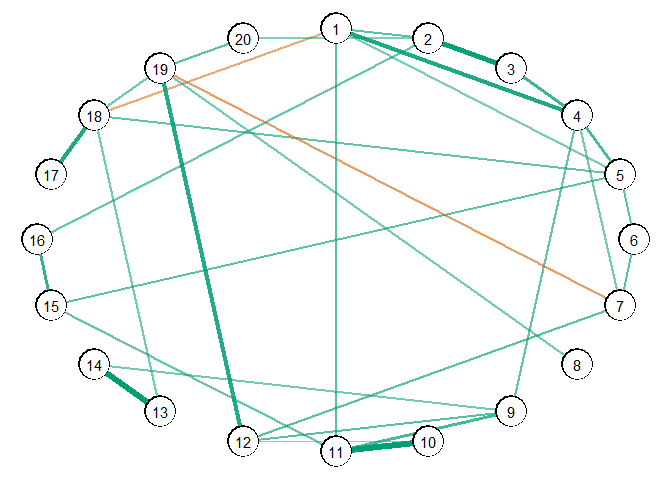
Bug reports and feature requests can be made by opening an issue on Github. To contribute towards the development of GGMnonreg, you can start a branch with a pull request and we can discuss the proposed changes there.
Epskamp, Sacha, Lourens J. Waldorp, Rene Mottus, and Denny Borsboom. 2018. “The Gaussian Graphical Model in Cross-Sectional and Time-Series Data.” Multivariate Behavioral Research 53 (4): 453–80. https://doi.org/10.1080/00273171.2018.1454823.
Marsman, M, D Borsboom, J Kruis, S Epskamp, R van Bork, L J Waldorp, By Taylor, L Waldorp, H L J van der Maas, and G Maris. 2017. “An Introduction to Network Psychometrics: Relating Ising Network Models to Item Response Theory Models.” Taylor & Francis 53 (1): 15–35. https://doi.org/10.1080/00273171.2017.1379379.
Williams, Donald R. 2020. “Learning to Live with Sampling Variability: Expected Replicability in Partial Correlation Networks.” PsyArXiv. https://doi.org/10.31234/osf.io/fb4sa.
Williams, Donald R., and Philippe Rast. 2019. “Back to the basics: Rethinking partial correlation network methodology.” British Journal of Mathematical and Statistical Psychology. https://doi.org/10.1111/bmsp.12173.
Williams, Donald R., Mijke Rhemtulla, Anna C Wysocki, and Philippe Rast. 2019. “On Nonregularized Estimation of Psychological Networks.” Multivariate Behavioral Research 54 (5): 719–50. https://doi.org/10.1080/00273171.2019.1575716.