![]()

abstr provides an R interface to the A/B Street
transport system simulation and network editing software. It provides
functions for converting origin-destination data, combined with data on
buildings representing origin and destination locations, into
.json files that can be directly imported into the A/B
Street city simulation.
See the formats page in the A/B Street documentation for details of the schema that the package outputs.
You can install the released version of abstr from CRAN with:
install.packages("abstr")Install the development version from GitHub as follows:
remotes::install_github("a-b-street/abstr")The example below shows how abstr can be used. The input
datasets include sf objects representing buildings,
origin-destination (OD) data represented as desire lines and
administrative zones representing the areas within which trips in the
desire lines start and end. With the exception of OD data, each of the
input datasets is readily available for most cities. The input datasets
are illustrated in the plots below, which show example data shipped in
the package, taken from the Seattle, U.S.
library(abstr)
library(tmap) # for map making
tm_shape(montlake_zones) + tm_polygons(col = "grey") +
  tm_shape(montlake_buildings) + tm_polygons(col = "blue")  +
tm_style("classic")
The map above is a graphical representation of the Montlake
residential neighborhood in central Seattle, Washington. Here,
montlake_zones represents neighborhood residential zones
declared by Seattle local government and montlake_buildings
being the accumulation of buildings listed in
OpenStreetMap
The final piece of the abstr puzzle is OD data.
head(montlake_od)
#> # A tibble: 6 × 6
#>    o_id  d_id Drive Transit  Bike  Walk
#>   <dbl> <dbl> <int>   <int> <int> <int>
#> 1   281   361    23       1     2    14
#> 2   282   361    37       4     0    11
#> 3   282   369    14       3     0     8
#> 4   301   361    27       4     3    15
#> 5   301   368     6       2     1    16
#> 6   301   369    14       2     0    13
In this example, the first two columns correspond to the origin and destination zones in Montlake, with the subsequent columns representing the transport mode share between these zones.
Let’s combine each of the elements outlined above, the zone, building
and OD data. We do this using the ab_scenario() function in
the abstr package, which generates a data frame
representing tavel between the montlake_buildings. While
the OD data contains information on origin and destination zone,
ab_scenario() ‘disaggregates’ the data and randomly selects
building within each origin and destination zone to simulate travel at
the individual level, as illustrated in the chunk below which uses only
a sample of the montlake_od data, showing travel between
three pairs of zones, to illustrate the process:
set.seed(42)
montlake_od_minimal = subset(montlake_od, o_id == "373" |o_id == "402" | o_id == "281" | o_id == "588" | o_id == "301" | o_id == "314")
output_sf = ab_scenario(
  od = montlake_od_minimal,
  zones = montlake_zones,
  zones_d = NULL,
  origin_buildings = montlake_buildings,
  destination_buildings = montlake_buildings,
  pop_var = 3,
  time_fun = ab_time_normal,
  output = "sf",
  modes = c("Walk", "Bike", "Drive", "Transit")
)
The output_sf object created above can be further
transformed to match A/B
Street’s schema and visualised in A/B Street, or visualised in R
(using the tmap package in the code chunk below):
tm_shape(output_sf) + tmap::tm_lines(col = "mode", lwd = .8, lwd.legeld.col = "black") +
  tm_shape(montlake_zones) + tmap::tm_borders(lwd = 1.2, col = "gray") +
  tm_text("id", size = 0.6) +
tm_style("cobalt")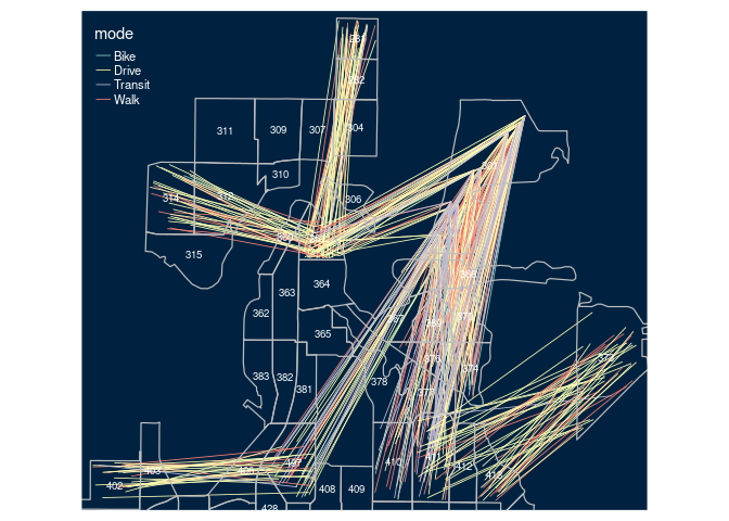
Each line in the plot above represents a single trip, with the color representing each transport mode. Moreover, each trip is configured with an associated departure time, that can be represented in A/B Street.
The ab_save and ab_json functions conclude
the abstr workflow by outputting a local JSON file,
matching the A/B
Street’s schema.
output_json = ab_json(output_sf, time_fun = ab_time_normal, scenario_name = "Montlake Example")
ab_save(output_json, f = "montlake.json")
Let’s see what is in the file:
file.edit("montlake.json")The first trip schedule should look something like this, matching A/B Street’s schema.
{
  "scenario_name": "Montlake Example",
  "people": [
    {
      "trips": [
        {
          "departure": 317760000,
          "origin": {
            "Position": {
              "longitude": -122.3139,
              "latitude": 47.667
            }
          },
          "destination": {
            "Position": {
              "longitude": -122.3187,
              "latitude": 47.6484
            }
          },
          "mode": "Walk",
          "purpose": "Shopping"
        }
      ]
    }
After generating a ab_scenario.json, you can import and
simulate it as follows.
ab_scenario.json
file.After you successfully import this file once, it will be available in
the list of scenarios, under the “Montlake Example” name, or whatever
name specified by the JSON file.
You can generate scenarios for any city in the world. See here for how to import new cities into A/B Street.
Note: Instead of installing a pre-built version of A/B Street in the
first step, feel free to build from
source, but it’s not necessary for any integration with the
abstr package.
If you’re generating many JSON scenarios, you might not want to manually use A/B Street’s user interface to import each file. You can instead run a command to do the import. See the docs at a-b-street.github.io/docs/tech/dev/ for details, but the basic steps are:
These steps can be achieved by running the following lines of code
(run the commented lines of code to install Rust, clone the A/B Street
repo and set the working directory, you can also replace
../montlake.json with a different path to the scenario
file):
# curl --proto '=https' --tlsv1.2 -sSf https://sh.rustup.rs | sh # install rust
# git clone git@github.com:a-b-street/abstreet
# cd abstreet
# cargo run --bin updater -- download --minimal
cargo run --bin cli -- import-scenario --input ../montlake.json --map data/system/us/seattle/maps/montlake.bin
cargo run --bin game --release
If you’re using Windows, you’ll instead run cli.exe. If
you’re building from source use the following command:
cargo run --release --bin cli -- import-scenario --input path/to/montlake.json --map data/system/us/seattle/maps/montlake.binFor a more comprehensive guide in the art of collecting, transforming
and saving data for A/B Street, check out the abstr documentation. The
package website, hosted at a-b-street.github.io/abstr,
contains articles that will help you get going with abstr.
See the following articles for reproducible examples that will help you
getting your valuable origin-destination and activity data into a
dynamic transport simulation environment for visualisation, model
exaperiments and more:
abstr
vignette for more detail on getting started with the package and
contextactivity
vignette on representing multi-trip-per-person activity models in R
and A/B Streetpct_to_abstr
vignette on importing output from an established project, the
Propensity to Cycle Tool, into A/B Street