This repo contains numerical implementations of algorithms to estimate weighted, undirected, (possibly k-component) bipartite graphs.
finbipartite depends on the development version of spectralGraphTopology.
You can install the development version from GitHub:
> devtools::install_github("convexfi/spectralGraphTopology")
> devtools::install_github("convexfi/finbipartite")On MS Windows environments, make sure to install the most recent
version of Rtools.
library(fitHeavyTail)
library(xts)
library(quantmod)
library(igraph)
library(finbipartite)
library(readr)
set.seed(42)
# load SP500 stock prices into an xts table
stock_prices <- readRDS("examples/stocks/sp500-data-2016-2021.rds")
# number of sectors
q <- 8
# number of stocks
r <- ncol(stock_prices) - q
# total nodes in the graph
p <- r + q
colnames(stock_prices)[1:r]
#> [1] "A" "AAL" "ABBV" "ABC" "ABMD" "ABT" "ADM" "AEE" "AEP" "AES"
#> [11] "AFL" "AIG" "AIV" "AIZ" "AJG" "ALB" "ALGN" "ALK" "ALL" "ALLE"
#> [21] "ALXN" "AMCR" "AME" "AMGN" "AMP" "AMT" "ANTM" "AON" "AOS" "APA"
#> [31] "APD" "ARE" "ATO" "AVB" "AVY" "AWK" "AXP" "BA" "BAC" "BAX"
#> [41] "BDX" "BEN" "BIIB" "BIO" "BK" "BKR" "BLK" "BLL" "BMY" "BSX"
#> [51] "BXP" "C" "CAG" "CAH" "CAT" "CB" "CBOE" "CBRE" "CCI" "CE"
#> [61] "CERN" "CF" "CFG" "CHD" "CHRW" "CI" "CINF" "CL" "CLX" "CMA"
#> [71] "CME" "CMI" "CMS" "CNC" "CNP" "COF" "COG" "COO" "COP" "COST"
#> [81] "COTY" "CPB" "CPRT" "CSX" "CTAS" "CVS" "CVX" "D" "DAL" "DD"
#> [91] "DE" "DFS" "DGX" "DHR" "DLR" "DOV" "DRE" "DTE" "DUK" "DVA"
#> [101] "DVN" "DXCM" "ECL" "ED" "EFX" "EIX" "EL" "EMN" "EMR" "EOG"
#> [111] "EQIX" "EQR" "ES" "ESS" "ETN" "ETR" "EVRG" "EW" "EXC" "EXPD"
#> [121] "EXR" "FANG" "FAST" "FBHS" "FCX" "FDX" "FE" "FITB" "FLS" "FMC"
#> [131] "FRC" "FRT" "FTI" "GD" "GE" "GILD" "GIS" "GL" "GS" "GWW"
#> [141] "HAL" "HBAN" "HCA" "HES" "HFC" "HIG" "HII" "HOLX" "HON" "HRL"
#> [151] "HSIC" "HST" "HSY" "HUM" "HWM" "ICE" "IDXX" "IEX" "IFF" "ILMN"
#> [161] "INCY" "INFO" "IP" "IQV" "IRM" "ISRG" "ITW" "IVZ" "J" "JBHT"
#> [171] "JCI" "JNJ" "JPM" "K" "KEY" "KHC" "KIM" "KMB" "KMI" "KO"
#> [181] "KR" "KSU" "L" "LH" "LHX" "LIN" "LLY" "LMT" "LNC" "LNT"
#> [191] "LUV" "LYB" "MAA" "MAS" "MCK" "MCO" "MDLZ" "MDT" "MET" "MKC"
#> [201] "MKTX" "MLM" "MMC" "MMM" "MNST" "MO" "MOS" "MPC" "MRK" "MRO"
#> [211] "MS" "MSCI" "MTB" "MTD" "NDAQ" "NEE" "NEM" "NI" "NLSN" "NOC"
#> [221] "NOV" "NRG" "NSC" "NTRS" "NUE" "O" "ODFL" "OKE" "OXY" "PBCT"
#> [231] "PCAR" "PEAK" "PEG" "PEP" "PFE" "PFG" "PG" "PGR" "PH" "PKG"
#> [241] "PKI" "PLD" "PM" "PNC" "PNR" "PNW" "PPG" "PPL" "PRGO" "PRU"
#> [251] "PSA" "PSX" "PWR" "PXD" "RE" "REG" "REGN" "RF" "RHI" "RJF"
#> [261] "RMD" "ROK" "ROL" "ROP" "RSG" "RTX" "SBAC" "SCHW" "SEE" "SHW"
#> [271] "SIVB" "SJM" "SLB" "SLG" "SNA" "SO" "SPG" "SPGI" "SRE" "STE"
#> [281] "STT" "STZ" "SWK" "SYF" "SYK" "SYY" "TAP" "TDG" "TDY" "TFC"
#> [291] "TFX" "TMO" "TROW" "TRV" "TSN" "TT" "TXT" "UAL" "UDR" "UHS"
#> [301] "UNH" "UNM" "UNP" "UPS" "URI" "USB" "VAR" "VLO" "VMC" "VNO"
#> [311] "VRSK" "VRTX" "VTR" "WAB" "WAT" "WBA" "WEC" "WELL" "WFC" "WLTW"
#> [321] "WM" "WMB" "WMT" "WRB" "WST" "WY" "XEL" "XOM" "XRAY" "XYL"
#> [331] "ZBH" "ZION" "ZTS"
colnames(stock_prices)[(r+1):p]
#> [1] "XLP" "XLE" "XLF" "XLV" "XLI" "XLB" "XLRE" "XLU"
selected_sectors <- c("Consumer Staples", "Energy", "Financials",
"Health Care", "Industrials", "Materials",
"Real Estate", "Utilities")
# compute log-returns
log_returns <- diff(log(stock_prices), na.pad = FALSE)
# fit an univariate Student-t distribution to the log-returns of the market
# to obtain an estimate of the degrees of freedom (nu)
mkt_index <- Ad(getSymbols("^GSPC",
from = index(stock_prices[1]), to = index(stock_prices[nrow(stock_prices)]),
auto.assign = FALSE,
verbose = FALSE))
mkt_index_log_returns <- diff(log(mkt_index), na.pad = FALSE)
nu <- fit_mvt(mkt_index_log_returns,
nu="MLE-diag-resampled")$nu
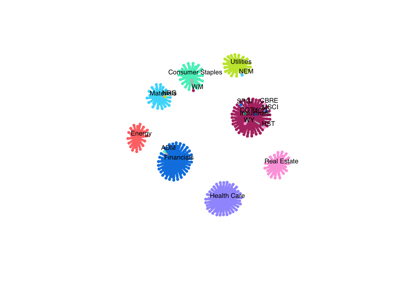
# learn a bipartite graph with k = 8 components
graph_mrf <- learn_heavy_tail_kcomp_bipartite_graph(scale(log_returns),
r = r,
q = q,
k = 8,
nu = nu,
learning_rate = 1,
verbose = FALSE)
# save predicted labels
labels_pred <- c()
for(i in c(1:r)){
labels_pred <- c(labels_pred, which.max(graph_mrf$B[i, ]))
}
# build network
SP500 <- read_csv("examples/stocks/SP500-sectors.csv")
stock_sectors <- SP500$GICS.Sector[SP500$Symbol %in% colnames(stock_prices)[1:r]]
stock_sectors_index <- as.numeric(as.factor(stock_sectors))
net <- graph_from_adjacency_matrix(graph_mrf$adjacency, mode = "undirected", weighted = TRUE)
colors <- c("#55efc4", "#ff7675", "#0984e3", "#a29bfe", "#B33771", "#48dbfb", "#FDA7DF", "#C4E538")
V(net)$color <- c(colors[stock_sectors_index], colors)
V(net)$type <- c(rep(FALSE, r), rep(TRUE, q))
V(net)$cluster <- c(stock_sectors_index, c(1:q))
E(net)$color <- apply(as.data.frame(get.edgelist(net)), 1,
function(x) ifelse(V(net)$cluster[x[1]] == V(net)$cluster[x[2]],
colors[V(net)$cluster[x[1]]], 'grey'))
# where do our predictions differ from GICS?
mask <- labels_pred != stock_sectors_index
node_labels <- colnames(stock_prices)[1:r]
node_labels[!mask] <- NA
# plot network
plot(net, vertex.size = c(rep(3, r), rep(5, q)),
vertex.label = c(node_labels, selected_sectors),
vertex.label.cex = 0.7, vertex.label.dist = 1.0,
vertex.frame.color = c(colors[stock_sectors_index], colors),
layout = layout_nicely(net),
vertex.label.family = "Helvetica", vertex.label.color = "black",
vertex.shape = c(rep("circle", r), rep("square", q)),
edge.width = 4*E(net)$weight)
If you made use of this software please consider citing: