
![]()
numform contains tools to assist in the formatting
of numbers and plots for publication. Tools include the removal of
leading zeros, standardization of number of digits, addition of affixes,
and a p-value formatter. These tools combine the functionality of
several ‘base’ functions such as paste(),
format(), and sprintf() into specific use case
functions that are named in a way that is consistent with usage, making
their names easy to remember and easy to deploy.
To download the development version of numform:
Download the zip ball or
tar
ball, decompress and run R CMD INSTALL on it, or use
the pacman package to install the development
version:
if (!require("pacman")) install.packages("pacman")
pacman::p_load_current_gh("trinker/numform")
pacman::p_load(tidyverse, gridExtra)You are welcome to:
- submit suggestions and bug-reports at: https://github.com/trinker/numform/issues
- send a pull request on: https://github.com/trinker/numform/
- compose a friendly e-mail to:
tyler.rinker@gmail.com
Below is a table of available numform functions.
Note that f_ is read as “format” whereas fv_
is read as “format vector”. The former formats individual values in the
vector while the latter uses the vector to compute a calculation on each
of the values and then formats them. Additionally, all
numform f_ functions have a closure,
function retuning, version that is prefixed with an additional
f (read “format function”). For example, f_num
has ff_num which has the same arguments but returns a
function instead. This is useful for passing in to
ggplot2 scale_x/y_type functions (see Plotting for usage).
| alignment | f_byte | f_latitude | f_peta | f_weekday_abbreviation |
| as_factor | f_celcius | f_list | f_pp | f_weekday_name |
| collapse | f_comma | f_list_amp | f_prefix | f_wrap |
| constant_months | f_data | f_logical | f_prop2percent | f_year |
| constant_months_abbreviation | f_data_abbreviation | f_longitude | f_pval | f_yotta |
| constant_quarters | f_date | f_mean_sd | f_quarter | f_zetta |
| constant_weekdays | f_degree | f_mega | f_replace | fv_num_percent |
| constant_weekdays_abbreviation | f_denom | f_mills | f_response | fv_percent |
| f_12_hour | f_dollar | f_month | f_sign | fv_percent_diff |
| f_abbreviation | f_exa | f_month_abbreviation | f_state | fv_percent_diff_fixed_relative |
| f_affirm | f_fahrenheit | f_month_name | f_suffix | fv_percent_lead |
| f_affix | f_giga | f_num | f_tera | fv_percent_lead_fixed_relative |
| f_bills | f_interval | f_num_percent | f_text_bar | fv_runs |
| f_bin | f_interval_right | f_ordinal | f_thous | glue |
| f_bin_right | f_interval_text | f_pad_zero | f_title | highlight_cells |
| f_bin_text | f_interval_text_right | f_parenthesis | f_trills | |
| f_bin_text_right | f_kilo | f_percent | f_weekday |
Available Formatting Functions
if (!require("pacman")) install.packages("pacman")
pacman::p_load_gh("trinker/numform")
pacman::p_load(dplyr)f_num(c(0.0, 0, .2, -00.02, 1.122222, pi, "A"))
## [1] ".0" ".0" ".2" "-.0" "1.1" "3.1" NAf_thous(1234)
## [1] "1K"
f_thous(12345)
## [1] "12K"
f_thous(123456)
## [1] "123K"
f_mills(1234567)
## [1] "1M"
f_mills(12345678)
## [1] "12M"
f_mills(123456789)
## [1] "123M"
f_bills(1234567891)
## [1] "1B"
f_bills(12345678912)
## [1] "12B"
f_bills(123456789123)
## [1] "123B"…or auto-detect:
f_denom(1234)

## [1] "1K"

f_denom(12345)

## [1] "12K"

f_denom(123456)

## [1] "123K"

f_denom(1234567)

## [1] "1M"

f_denom(12345678)

## [1] "12M"

f_denom(123456789)

## [1] "123M"

f_denom(1234567891)

## [1] "1B"

f_denom(12345678912)

## [1] "12B"

f_denom(123456789123)

## [1] "123B"f_comma(c(1234.12345, 1234567890, .000034034, 123000000000, -1234567))
## [1] "1,234.123" "1,234,567,890" ".000034034" "123,000,000,000"
## [5] "-1,234,567"f_percent(c(30, 33.45, .1), digits = 1)
## [1] "30.0%" "33.5%" ".1%"
f_percent(c(0.0, 0, .2, -00.02, 1.122222, pi))
## [1] ".0%" ".0%" ".2%" "-.0%" "1.1%" "3.1%"
f_prop2percent(c(.30, 1, 1.01, .33, .222, .01))
## [1] "30.0%" "100.0%" "101.0%" "33.0%" "22.2%" "1.0%"
f_prop2percent(c(.30, 1, 1.01, .33, .222, .01), digits = 0)
## [1] "30%" "100%" "101%" "33%" "22%" "1%"
f_pp(c(.30, 1, 1.01, .33, .222, .01)) # same as f_prop2percent(digits = 0)
## [1] "30%" "100%" "101%" "33%" "22%" "1%"f_dollar(c(0, 30, 33.45, .1))
## [1] "$0.00" "$30.00" "$33.45" "$0.10"
f_dollar(c(0.0, 0, .2, -00.02, 1122222, pi)) %>%
f_comma()
## [1] "$0.00" "$0.00" "$0.20" "$-.02"
## [5] "$1,122,222.00" "$3.14"Sometimes one wants to lop off digits of money in order to see the
important digits, the real story. The f_denom family of
functions can do job.
f_denom(c(12345267, 98765433, 658493021), prefix = '$')

## [1] "$ 12M" "$ 99M" "$658M"

f_denom(c(12345267, 98765433, 658493021), relative = 1, prefix = '$')

## [1] "$ 12.3M" "$ 98.8M" "$658.5M"Notice the use of the alignment function to detect the
column alignment.
pacman::p_load(dplyr, pander)
set.seed(10)
dat <- data_frame(
Team = rep(c("West Coast", "East Coast"), each = 4),
Year = rep(2012:2015, 2),
YearStart = round(rnorm(8, 2e6, 1e6) + sample(1:10/100, 8, TRUE), 2),
Won = round(rnorm(8, 4e5, 2e5) + sample(1:10/100, 8, TRUE), 2),
Lost = round(rnorm(8, 4.4e5, 2e5) + sample(1:10/100, 8, TRUE), 2),
WinLossRate = Won/Lost,
PropWon = Won/YearStart,
PropLost = Lost/YearStart
)
dat %>%
group_by(Team) %>%
mutate(
`%ΔWinLoss` = fv_percent_diff(WinLossRate, 0),
`ΔWinLoss` = f_sign(Won - Lost, '<b>+</b>', '<b>–</b>')
) %>%
ungroup() %>%
mutate_at(vars(Won:Lost), .funs = ff_denom(relative = -1, prefix = '$')) %>%
mutate_at(vars(PropWon, PropLost), .funs = ff_prop2percent(digits = 0)) %>%
mutate(
YearStart = f_denom(YearStart, 1, prefix = '$'),
Team = fv_runs(Team),
WinLossRate = f_num(WinLossRate, 1)
) %>%
data.frame(stringsAsFactors = FALSE, check.names = FALSE) %>%
pander::pander(split.tables = Inf, justify = alignment(.), style = 'simple')| Team | Year | YearStart | Won | Lost | WinLossRate | PropWon | PropLost | %ΔWinLoss | ΔWinLoss | ||
|---|---|---|---|---|---|---|---|---|---|---|---|
| West Coast | 2012 | $2.0M | $350K | $190K | 1.9 | 17% | 9% | 0% | + | ||
| 2013 | $1.8M | $600K | \(370K</td> <td align="right">1.6</td> <td align="right">33%</td> <td align="right">20%</td> <td align="right">-13%</td> <td align="right"><b>+</b></td> </tr> <tr class="odd"> <td align="left"></td> <td align="right">2014</td> <td align="right">\) .6M | $550K | $300K | 1.8 | 87% | 48% | 11% | + | |
| 2015 | $1.4M | $420K | $270K | 1.6 | 30% | 19% | -13% | + | |||
| East Coast | 2012 | $2.3M | $210K | $420K | .5 | 9% | 18% | 0% | – | ||
| 2013 | $2.4M | $360K | \(390K</td> <td align="right">.9</td> <td align="right">15%</td> <td align="right">16%</td> <td align="right">86%</td> <td align="right"><b>–</b></td> </tr> <tr class="odd"> <td align="left"></td> <td align="right">2014</td> <td align="right">\) .8M | \(590K</td> <td align="right">\) 70K | 8.4 | 74% | 9% | 811% | + | ||
| 2015 | $1.6M | $500K | $420K | 1.2 | 30% | 26% | -86% | + |
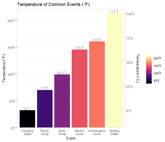
pacman::p_load(dplyr, pander)

data_frame(
    Event = c('freezing water', 'room temp', 'body temp', 'steak\'s done', 'hamburger\'s done', 'boiling water', 'sun surface', 'lighting'),
    F = c(32, 70, 98.6, 145, 160, 212, 9941, 50000)
) %>%
    mutate(
        Event = f_title(Event),
        C = (F - 32) * (5/9)
    ) %>%
    mutate(
        F = f_degree(F, measure = 'F', type = 'string'),
        C = f_degree(C, measure = 'C', type = 'string', zero = '0.0')
    )  %>%
    data.frame(stringsAsFactors = FALSE, check.names = FALSE) %>%
pander::pander(split.tables = Inf, justify = alignment(.), style = 'simple')| Event | F | C |
|---|---|---|
| Freezing Water | 32.0°F | 0.0°C |
| Room Temp | 70.0°F | 21.1°C |
| Body Temp | 98.6°F | 37.0°C |
| Steak’s Done | 145.0°F | 62.8°C |
| Hamburger’s Done | 160.0°F | 71.1°C |
| Boiling Water | 212.0°F | 100.0°C |
| Sun Surface | 9941.0°F | 5505.0°C |
| Lighting | 50000.0°F | 27760.0°C |
if (!require("pacman")) install.packages("pacman")
pacman::p_load(tidyverse)

set.seed(11)
data_frame(
    date = sample(seq(as.Date("1990/1/1"), by = "day", length.out = 2e4), 12)
) %>%
    mutate(
        year_4 = f_year(date, 4),
        year_2 = f_year(date, 2),
        quarter = f_quarter(date),
        month_name = f_month_name(date) %>%
            numform::as_factor(),
        month_abbreviation = f_month_abbreviation(date) %>%
            numform::as_factor(),
        month_short = f_month(date),
        weekday_name = f_weekday_name(date),
        weekday_abbreviation = f_weekday_abbreviation(date),
       weekday_short = f_weekday(date),
        weekday_short_distinct = f_weekday(date, distinct = TRUE)
    ) %>%
    data.frame(stringsAsFactors = FALSE, check.names = FALSE) %>%
pander::pander(split.tables = Inf, justify = alignment(.), style = 'simple')| date | year_4 | year_2 | quarter | month_name | month_abbreviation | month_short | weekday_name | weekday_abbreviation | weekday_short | weekday_short_distinct |
|---|---|---|---|---|---|---|---|---|---|---|
| 2005-03-07 | 2005 | 05 | Q1 | March | Mar | M | Monday | Mon | M | M |
| 1990-01-11 | 1990 | 90 | Q1 | January | Jan | J | Thursday | Thu | T | Th |
| 2017-12-16 | 2017 | 17 | Q4 | December | Dec | D | Saturday | Sat | S | S |
| 1990-10-08 | 1990 | 90 | Q4 | October | Oct | O | Monday | Mon | M | M |
| 1993-07-17 | 1993 | 93 | Q3 | July | Jul | J | Saturday | Sat | S | S |
| 2042-04-10 | 2042 | 42 | Q2 | April | Apr | A | Thursday | Thu | T | Th |
| 1994-09-26 | 1994 | 94 | Q3 | September | Sep | S | Monday | Mon | M | M |
| 2005-11-15 | 2005 | 05 | Q4 | November | Nov | N | Tuesday | Tue | T | T |
| 2038-03-16 | 2038 | 38 | Q1 | March | Mar | M | Tuesday | Tue | T | T |
| 1996-09-29 | 1996 | 96 | Q3 | September | Sep | S | Sunday | Sun | S | Su |
| 1999-08-02 | 1999 | 99 | Q3 | August | Aug | A | Monday | Mon | M | M |
| 2014-02-14 | 2014 | 14 | Q1 | February | Feb | F | Friday | Fri | F | F |
mtcars %>%
    count(cyl, gear) %>%
    group_by(cyl) %>%
    mutate(
        p = numform::f_pp(n/sum(n))
    ) %>%
    ungroup() %>%
    mutate(
        cyl = numform::fv_runs(cyl),
        ` ` = f_text_bar(n)  ## Overall
    ) %>%
    as.data.frame()

  cyl gear  n   p
1   4    3  1  9% _
2        4  8 73% ______
3        5  2 18% __
4   6    3  2 29% __
5        4  4 57% ___
6        5  1 14% _
7   8    3 12 86% _________
8 5 2 14% __ library(tidyverse); library(viridis)
set.seed(10)
data_frame(
revenue = rnorm(10000, 500000, 50000),
date = sample(seq(as.Date('1999/01/01'), as.Date('2000/01/01'), by="day"), 10000, TRUE),
site = sample(paste("Site", 1:5), 10000, TRUE)
) %>%
mutate(
dollar = f_comma(f_dollar(revenue, digits = -3)),
thous = f_denom(revenue),
thous_dollars = f_denom(revenue, prefix = '$'),
abb_month = f_month(date),
abb_week = numform::as_factor(f_weekday(date, distinct = TRUE))
) %>%
group_by(site, abb_week) %>%
mutate(revenue = {if(sample(0:1, 1) == 0) `-` else `+`}(revenue, sample(1e2:1e5, 1))) %>%
ungroup() %T>%
print() %>%
ggplot(aes(abb_week, revenue)) +
geom_jitter(width = .2, height = 0, alpha = .2, aes(color = revenue)) +
scale_y_continuous(label = ff_denom(prefix = '$'))+
facet_wrap(~site) +
theme_bw() +
scale_color_viridis() +
theme(
strip.text.x = element_text(hjust = 0, color = 'grey45'),
strip.background = element_rect(fill = NA, color = NA),
panel.border = element_rect(fill = NA, color = 'grey75'),
panel.grid = element_line(linetype = 'dotted'),
axis.ticks = element_line(color = 'grey55'),
axis.text = element_text(color = 'grey55'),
axis.title.x = element_text(color = 'grey55', margin = margin(t = 10)),
axis.title.y = element_text(color = 'grey55', angle = 0, margin = margin(r = 10)),
legend.position = 'none'
) +
labs(
x = 'Day of Week',
y = 'Revenue',
title = 'Site Revenue by Day of Week',
subtitle = f_wrap(c(
'This faceted dot plot shows the distribution of revenues within sites',
'across days of the week. Notice the consistently increasing revenues for',
'Site 2 across the week.'
), width = 85, collapse = TRUE)
)
## # A tibble: 10,000 x 8
## revenue date site dollar thous thous_dollars abb_month abb_week
## <dbl> <date> <chr> <chr> <chr> <chr> <chr> <fct>
## 1 449648. 1999-11-29 Site 1 $501,0~ 501K $501K N M
## 2 560514. 1999-07-07 Site 4 $491,0~ 491K $491K J W
## 3 438891. 1999-08-06 Site 2 $431,0~ 431K $431K A F
## 4 528543. 1999-05-04 Site 3 $470,0~ 470K $470K M T
## 5 462758. 1999-07-08 Site 4 $515,0~ 515K $515K J Th
## 6 553879. 1999-07-22 Site 2 $519,0~ 519K $519K J Th
## 7 473985. 1999-05-20 Site 2 $440,0~ 440K $440K M Th
## 8 533825. 1999-05-28 Site 5 $482,0~ 482K $482K M F
## 9 426124. 1999-01-15 Site 2 $419,0~ 419K $419K J F
## 10 406613. 1999-08-19 Site 3 $487,0~ 487K $487K A Th
## # ... with 9,990 more rows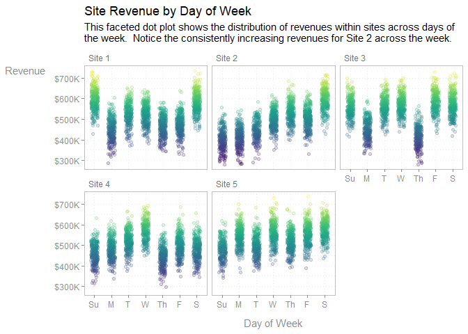
library(tidyverse); library(viridis)
set.seed(10)
dat <- data_frame(
revenue = rnorm(144, 500000, 10000),
date = seq(as.Date('2005/01/01'), as.Date('2016/12/01'), by="month")
) %>%
mutate(
quarter = f_quarter(date),
year = f_year(date, 4)
) %>%
group_by(year, quarter) %>%
summarize(revenue = sum(revenue)) %>%
ungroup() %>%
mutate(quarter = as.integer(gsub('Q', '', quarter)))
year_average <- dat %>%
group_by(year) %>%
summarize(revenue = mean(revenue)) %>%
mutate(x1 = .8, x2 = 4.2)
dat %>%
ggplot(aes(quarter, revenue, group = year)) +
geom_segment(
linetype = 'dashed',
data = year_average, color = 'grey70', size = 1,
aes(x = x1, y = revenue, xend = x2, yend = revenue)
) +
geom_line(size = .85, color = '#009ACD') +
geom_point(size = 1.5, color = '#009ACD') +
facet_wrap(~year, nrow = 2) +
scale_y_continuous(label = ff_denom(relative = 2)) +
scale_x_continuous(breaks = 1:4, label = f_quarter) +
theme_bw() +
theme(
strip.text.x = element_text(hjust = 0, color = 'grey45'),
strip.background = element_rect(fill = NA, color = NA),
panel.border = element_rect(fill = NA, color = 'grey75'),
panel.grid.minor = element_blank(),
panel.grid.major = element_line(linetype = 'dotted'),
axis.ticks = element_line(color = 'grey55'),
axis.text = element_text(color = 'grey55'),
axis.title.x = element_text(color = 'grey55', margin = margin(t = 10)),
axis.title.y = element_text(color = 'grey55', angle = 0, margin = margin(r = 10)),
legend.position = 'none'
) +
labs(
x = 'Quarter',
y = 'Revenue ($)',
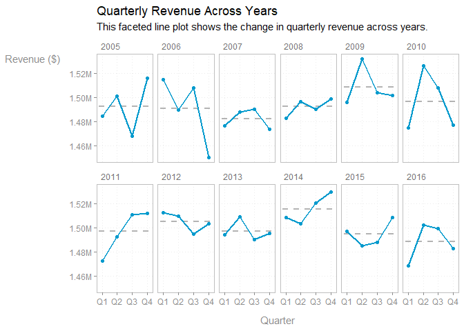
title = 'Quarterly Revenue Across Years',
subtitle = f_wrap(c(
'This faceted line plot shows the change in quarterly revenue across',
'years.'
), width = 85, collapse = TRUE)
)
library(tidyverse); library(gridExtra)
set.seed(10)
dat <- data_frame(
level = c("not_involved", "somewhat_involved_single_group",
"somewhat_involved_multiple_groups", "very_involved_one_group",
"very_involved_multiple_groups"
),
n = sample(1:10, length(level))
) %>%
mutate(
level = factor(level, levels = unique(level)),
`%` = n/sum(n)
)
gridExtra::grid.arrange(
gridExtra::arrangeGrob(
dat %>%
ggplot(aes(level, `%`)) +
geom_col() +
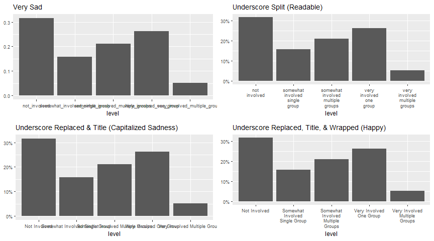
labs(title = 'Very Sad', y = NULL) +
theme(
axis.text = element_text(size = 7),
title = element_text(size = 9)
),
dat %>%
ggplot(aes(level, `%`)) +
geom_col() +
scale_x_discrete(labels = function(x) f_replace(x, '_', '\n')) +
scale_y_continuous(labels = ff_prop2percent(digits = 0)) +
labs(title = 'Underscore Split (Readable)', y = NULL) +
theme(
axis.text = element_text(size = 7),
title = element_text(size = 9)
),
ncol = 2
),
gridExtra::arrangeGrob(
dat %>%
ggplot(aes(level, `%`)) +
geom_col() +
scale_x_discrete(labels = function(x) f_title(f_replace(x))) +
scale_y_continuous(labels = ff_prop2percent(digits = 0)) +
labs(title = 'Underscore Replaced & Title (Capitalized Sadness)', y = NULL) +
theme(
axis.text = element_text(size = 7),
title = element_text(size = 9)
),
dat %>%
ggplot(aes(level, `%`)) +
geom_col() +
scale_x_discrete(labels = function(x) f_wrap(f_title(f_replace(x)))) +
scale_y_continuous(labels = ff_prop2percent(digits = 0)) +
labs(title = 'Underscore Replaced, Title, & Wrapped (Happy)', y = NULL) +
theme(
axis.text = element_text(size = 7),
title = element_text(size = 9)
),
ncol = 2
), ncol = 1
)
set.seed(10)
dat <- data_frame(
state = sample(state.name, 10),
value = sample(10:20, 10) ^ (7),
cols = sample(colors()[1:150], 10)
) %>%
arrange(desc(value)) %>%
mutate(state = factor(state, levels = unique(state)))
dat %>%
ggplot(aes(state, value, fill = cols)) +
geom_col() +
scale_x_discrete(labels = f_state) +
scale_fill_identity() +
scale_y_continuous(labels = ff_denom(prefix = '$'), expand = c(0, 0),
limits = c(0, max(dat$value) * 1.05)
) +
theme_minimal() +
theme(
panel.grid.major.x = element_blank(),
axis.title.y = element_text(angle = 0)
) +
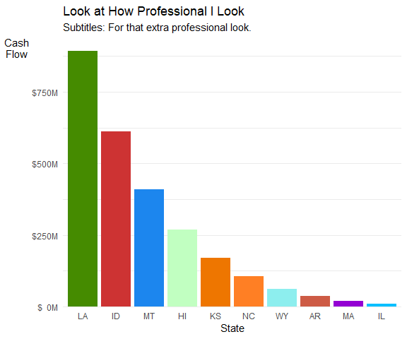
labs(x = 'State', y = 'Cash\nFlow',
title = f_title("look at how professional i look"),
subtitle = 'Subtitles: For that extra professional look.'
)
library(tidyverse); library(viridis)

data_frame(
    Event = c('freezing water', 'room temp', 'body temp', 'steak\'s done', 'hamburger\'s done', 'boiling water'),
    F = c(32, 70, 98.6, 145, 160, 212)
) %>%
    mutate(
        C = (F - 32) * (5/9),
        Event = f_title(Event),
        Event = factor(Event, levels = unique(Event))
    ) %>%
    ggplot(aes(Event, F, fill = F)) +
        geom_col() +
        geom_text(aes(y = F + 4, label = f_fahrenheit(F, digits = 1, type = 'text')), parse = TRUE, color = 'grey60') +
        scale_y_continuous(
            labels = f_fahrenheit, limits = c(0, 220), expand = c(0, 0),
            sec.axis = sec_axis(trans = ~(. - 32) * (5/9), labels = f_celcius, name = f_celcius(prefix = 'Temperature ', type = 'title'))
        ) +
        scale_x_discrete(labels = ff_replace(pattern = ' ', replacement = '\n')) +
        scale_fill_viridis(option =  "magma", labels = f_fahrenheit, name = NULL) +
        theme_bw() +
        labs(
            y = f_fahrenheit(prefix = 'Temperature ', type = 'title'),
            title = f_fahrenheit(prefix = 'Temperature of Common Events ', type = 'title')
        ) +
        theme(
            axis.ticks.x = element_blank(),
            panel.border = element_rect(fill = NA, color = 'grey80'),
            panel.grid.minor.x = element_blank(),
            panel.grid.major.x = element_blank()
        )
library(tidyverse); library(maps)

world <- map_data(map="world")

ggplot(world, aes(map_id = region, x = long, y = lat)) +
    geom_map(map = world, aes(map_id = region), fill = "grey40", colour = "grey70", size = 0.25) +
    scale_y_continuous(labels = f_latitude) +
    scale_x_continuous(labels = f_longitude)
mtcars %>%
    mutate(mpg2 = cut(mpg, 10, right = FALSE)) %>%
    ggplot(aes(mpg2)) +
        geom_bar(fill = '#33A1DE') +
        scale_x_discrete(labels = function(x) f_wrap(f_bin_text_right(x, l = 'up to'), width = 8)) +
        scale_y_continuous(breaks = seq(0, 14, by = 2), limits = c(0, 7)) +
        theme_minimal() +
        theme(
            panel.grid.major.x = element_blank(),
            axis.text.x = element_text(size = 14, margin = margin(t = -12)),
            axis.text.y = element_text(size = 14),
            plot.title = element_text(hjust = .5)
        ) +
        labs(title = 'Histogram', x = NULL, y = NULL)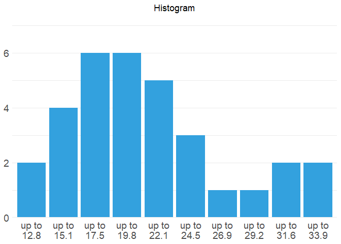
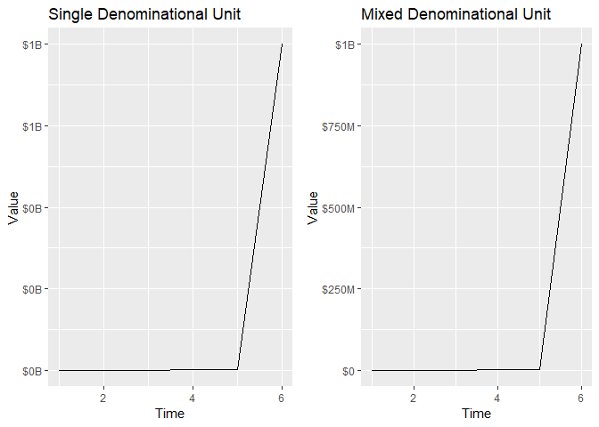
dat <- data_frame(
    Value = c(111, 2345, 34567, 456789, 1000001, 1000000001),
    Time = 1:6
)

gridExtra::grid.arrange(

    ggplot(dat, aes(Time, Value)) +
        geom_line() +
        scale_y_continuous(labels = ff_denom( prefix = '$')) +
        labs(title = "Single Denominational Unit"),

    ggplot(dat, aes(Time, Value)) +
        geom_line() +
        scale_y_continuous(
            labels = ff_denom(mix.denom = TRUE, prefix = '$', pad.char = '')
        ) +
        labs(title = "Mixed Denominational Unit"),

    ncol = 2
)
We can see its use in actual model reporting as well:
mod1 <- t.test(1:10, y = c(7:20))

sprintf(
    "t = %s (%s)",
    f_num(mod1$statistic),
    f_pval(mod1$p.value)
)

## [1] "t = -5.4 (p < .05)"

mod2 <- t.test(1:10, y = c(7:20, 200))

sprintf(
    "t = %s (%s)",
    f_num(mod2$statistic, 2),
    f_pval(mod2$p.value, digits = 2)
)

## [1] "t = -1.63 (p = .12)"
We can build a function to report model statistics:
report <- function(mod, stat = NULL, digits = c(0, 2, 2)) {
stat <- if (is.null(stat)) stat <- names(mod[["statistic"]])
sprintf(
"%s(%s) = %s, %s",
gsub('X-squared', 'Χ<sup>2</sup>', stat),
paste(f_num(mod[["parameter"]], digits[1]), collapse = ", "),
f_num(mod[["statistic"]], digits[2]),
f_pval(mod[["p.value"]], digits = digits[3])
)
}
report(mod1)
## [1] "t(22) = -5.43, p < .05"
report(oneway.test(count ~ spray, InsectSprays))
## [1] "F(5, 30) = 36.07, p < .05"
report(chisq.test(matrix(c(12, 5, 7, 7), ncol = 2)))
## [1] "Χ<sup>2</sup>(1) = .64, p = .42"This enables in-text usage as well. First set up the models in a code chunk:
mymod <- oneway.test(count ~ spray, InsectSprays)
mymod2 <- chisq.test(matrix(c(12, 5, 7, 7), ncol = 2))
And then use `r report(mymod)`